Regression

What is Regression?

scribble

• regression going back to the mean.
• height of the people is kind of a random walk to some extent.

slides

transcript

M: So, let me tell you about regression. We are in this section of the class, talking about supervised learning. In supervised learning we can take examples of inputs and outputs and based on that we are going to be able to take a new input and predict the corresponding output for that input, right. We are going to be talking about mapping continuous inputs to outputs. As opposed to, what was the other thing that we were mapping, what other kinds of outputs did we think about?

C: Well, we had discrete outputs and continuous outputs.

M: Right, and so this is going to be the focus on continuous. So regression seems like sort of an odd word. It doesn’t really kind of fit for this. So often I think about regression as. So this is, this is me being all sad and sort of reverting back to a childhood state. And that’s, you know, that’s in the psychological sense, that’s what regression refers to. But it turns out that, that’s not what it means in this setting. But the story by which those things became linked, I think, is kind of interesting. So let me tell you about that. Okay. So, this is a picture of you Charles. You can tell it’s you because he’s really tall.And you’re, you’re a fairly tall man. I know you don’t think of yourself that way, but you think of everyone else as being short which is really the same thing. So let’s say that this is Charles. Let’s say that this is someone of average height. Just someone at random. Now, let’s pretend that you have children.

C: I do have children.

M: All right. Okay but we can just pretend, and we want to ask the question what would you expect the average height of your children to be? Would you expect it to be sort of, you know, sort of Charles’ height? Or average height or may be somewhere between.

M: Okay Charles, so what do you think about this? Let’s say that their adult height is going to be a little bit smaller than you. So the average height of your children, you would you say it would be like an average height person? Or like your height or sort of in between?

C: In between. M: In between. All right. So it turns out that if you actually do this, you measure people’s heights and you measure the heights of their children, that that is in fact what you tend to see. That very, very tall people, like you tend to have taller than average children. But the height is between. It actually regresses to the mean. And here we really do mean regresses in the sense of going back to this kind of more primitive state that, if you think about average height people, as being like your ancestors, then, you know, you as a, as a very tall person tend to have kids that that tend regress back toward that average value that sort of, more older, more ancient value. So does that that make some sense to you?

C: That makes some sense. But one comment and one question. Comment, that is awesome because I’ve always actually wondered what regresses to the mean actually means. The second, what prevents us from all being the same height then?

M: Yes, so what, what seems to be happening is that there’s a kind of a noisy process and some people turn out to be taller, but then the next generation there’s a little bit of a history effect in people stay taller, but it tends to drift back towards the mean. So its sort of like a random walk, to some extent.

C: Oh, that actually kind of makes sense.

Regression and Function Approximation

scribble

• Regression means functional form of approximation towards the mean.

slides

transcript

M: Alright, so what does this have to do with function approximation or regression. So how does this notion of regression of falling back toward the mean have to do with this idea of approximating functions, mapping inputs to outputs, it seems kind of odd. So’m going to draw a graph and on this axis will be the parent height. And on this axis will be the average child height. So if we plot these against each other, let’s let me put the mean up here. Let’s say that this is mean height for the population. And now say that you know pair, we sort of imagine that parents of average height will have children of average height. But parents that are really tall, like that hypothetical person from before, will have children that are taller than average but not as tall as themselves. And similarly people that are very let’s say of smaller stature will have children that are also you know short. And, but not quite as short again closer to the mean. And it turns out that you have this, this very nice linear relationship between these quantities, and, there’s an important aspect to this. Which is that the slope of this line is less than one, it’s two thirds. Right. If the slope of this line was one, what would that mean Charles?

C: That would mean that everybody’s children would height of their parents.

M: Right, right, and so that’s exactly right. If this slope is less than one, like it is, it turns out to be in real populations. Then what’s happening is the children are little shorter than the parents. Children of taller parents are shorter than they are. And the children of short parents are taller than they are. And that’s the fact that this is less than one is what makes it regression to the mean. Now this, this was worked out in I believe in the late 1800s and it was just such a beautiful way of connecting all these different quantities together. To kind of think of them as being related in this functional way. That people said, oh this is really great. I’m going to use this idea of regression. And what they started to mean actually was this not this idea of regression to the mean. But this idea of finding a mathematical relationship based on a bunch of measurements of points. So this term ended up getting misused. But that’s the term that we have now. So regression now refers to not this idea of collapsing back towards the mean, but the idea of using functional form to approximate a bunch of data points. Isn’t that weird. There’s another example of this sort of idea where where a reasonable word, like, like regression which we’re referring to some physical thing in the, in the world due to experiments like psych experiments at this point became this mathematical concept where the name doesn’t really fit anymore, like there isn’t really anything regressing in what we’re doing. Do you do you know what I’m thinking of Charles?

C: No.

M: So reinforcement learning is my field of study. And it turns out that reinforcement learning doesn’t mean what the word means anymore. That this was a concept that the psychologist used to explain what they were observing. And then some mathematicians, well let’s call them computer scientists, took the word themselves, started to use it and used it wrong, but now it stuck and regression is another example like that. The word is sort of being used wrong, but it stuck and that’s what we’re going to use.

Linear Regression

scribble

• A linear function does not capture the data right.
• The linear relationship was designed which reduces the root mean square error.

slides

transcript

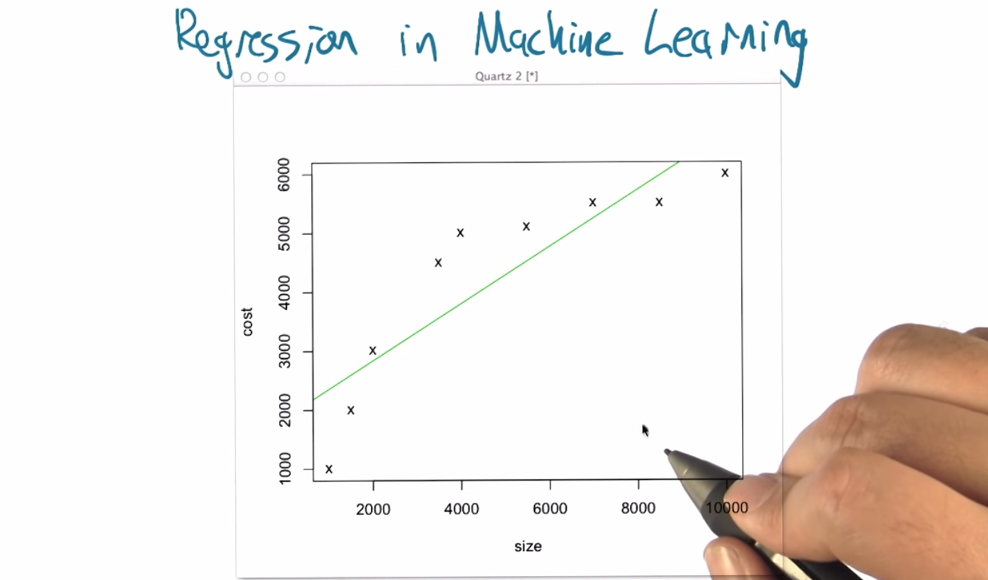
M: Alright, so, one of the things that’s very helpful about regression is that in many ways it’s very simple to visualize, it’s very simple to think about what some of the issues are and all the various topics in machine learning that are really important to understand and sometimes are difficult concepts really do come up in a fairly easy to understand way. So what I’d like to do now is to step through an example Of doing some regression and to point out what some of the pitfalls are and how they’re generally handled in the machine learning context. So, this graph that I put up here, is, we just made these numbers up, but it’s supposed to tell us a, a little bit about housing prices. So let’s imagine that we’re off to buy a house and what we notice is that there’s lots of different houses on the market, and there are lots of different, sizes, right. So ,the square footage of the house can vary. And in this case the houses that I visited can be between, about 1,000 to 10,000 square feet. And of course, as you get bigger houses, you tend to get more, the prices tend to go up too. Alright, so the price that the house cost tends to rise with the size of the house. So, what I’ve done here is I’ve plotted as a little x say a set of nine houses that I’ve observed. Start off over here with a house that’s a 1,000 square feet and cost a $1,000? I don’t know what year this happened in. And we end up with a house that is 10,000 square feet and cost about $6,000. So imagine that this is the relationship we observe. But now we want to answer a question like, Well, what happens If we find a house on the market and it’s about $5,000, what do you think a fair price for that would be? So what do you, what do you think, Charles? Looking at this, what do you think a fair price for a 5,000 square foot house would be?

C: Apparently about $5,000.

M: About, $5,000. Right. So, how did you do that?

C: I looked at the graph, I went over to 5,000 square feet at the x-axis and I went up. Until I found ,where one of the x’s was on the y axis and I said, oh, that’s about 5,000 square feet.

M: Well, but there was no corresponding point for that, so you had to interpolate or something based on the points that were there you had to kind of imagine what might, happening at the 5,000 square foot mark, right?

C: That’s true, although this one was a little easy because at 4,000 and 6,000 square feet, they were almost exactly the same so that, to you, made it feel like there was probably the level where things in this range would be. Alright, that seems kind of reasonable. So sure, though what we’re going to do in this case is actually try to find a, a function that fits this. Alright, well what if there is a linear relationship? What would be the best linear function that captures the relationship between the size and the cost. So what I have here is, it turns out of all the possible linear functions, this is the one that minimizes the squared error, the squared deviation, between these x points and the corresponding position on green line. So it finds a way of balancing all those different errors against each other and that’s the best line we’ve got. Now in this particular case, it’s interesting right, because if you put your idea of 5,000 square feet. Look what this line predicts. It’s something more like $4,000, right. Do you see that?

M: I do. That is doesn’t seem right to me.

C: It doesn’t, yeah, it doesn’t really look like a very good fit. But it does at least capture the fact that there is increasing cost with, with increase in size.

M: That’s true.

Finding the Best Fit

scribble

• Error is defined as sum of the distances between the x points and the green line.
• Many different error functions. We could use any of it.
• We use squared error as we can use calculus to find mininum error value.

slides

transcript

Alright. So it’s worth asking, how do we find this best line? So again there’s an infinite number of lines. How do we find one that fits these points the best. And again we’re defining best fit. As the one that has the least squared error, where the error is going to be some of the distances between these x points and the green line that we, that we fit. I’m not even sure that this really is the best fit in this case. I just kind of hand drew it. So is this something that we would want to solve by hill climbing which is to say we kind of the slope and the intercept of the line and we just kind of try different values of this until it gets better and better and then we can’t get any better and we stop. Can we do this using calculus? Can we use random search, where we just like, pick a random M, pick a random B, and see if we’re happy with it? Or is this the sort of thing where we probably would just go and ask a physicist because it involves, like, continuous quantities, and we’re discreet people?

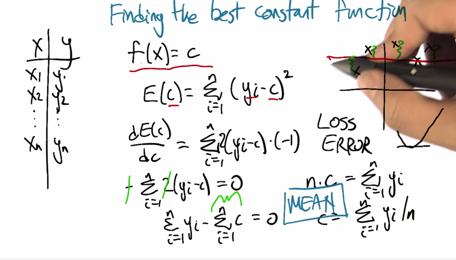
M: So let’s actually go through that exercise and derive how we do that. because it’s not so bad in two dimensions and it generalizes to higher dimensions as well. So it turns out that we can use calculus to do this, I am not going to step through the two-variable example for reasons that I am embarrassed to say. But I am going to show you a different example. So imagine that what we’re trying to do is that we’ve got a bunch of data points, and we’re trying to find the best constant function, right? So the best function that has the form, the value of the function for any given X is always the same constant,

C. So if our data looks like this, we got a bunch of X’s and a bunch of Y’s, then what we’re going to do, we’re going to say for any given value of C, any given constant, we can have an error. What’s the error going to be? The error is going to be the sum over all of the data points. Speaker 1: The square difference between that constant we chose and what the actual y value is.

C: Can I ask you a question? Why are we doing sum of squares?

M: There is many different error functions and sometimes called a relative concept called the loss function. There is lots of different ones that could work. You can do the absolute error, you can do the squared error, you can do various kinds of squashed errors where you know. The errors count different depending on how, how much deviation there is. It turns out that this one is particularly well behaved because of this reason that I’m explaining now that that because this error function is smooth as a function of the constant C, we can use calculus to actually find the minimum error value. But there’s lots of other things that could work and they actually do find utility in various different machine learning settings. So just now using the chain rule, if you want to find how do this error function output change as a function of input c. We can take the derivative of this sum you know, bring the two over. Times this, times the derivative of the inside, which is negative one in this case. And now this gives us a nice, smooth function saying what the error is as a function of c. And if we want to find the minimum, what do we want to do to this quantity?

C: Set it equal to zero, because that’s what I remember from Calculus.

M: That’s right. So in particular if the error you know, the error function is a nice smooth thing the derivative is negative and then zero and then positive. When it hits zero that’s when the thing has bottomed-out. Alright. So now we just need to solve this, this equation for c. So we have one equation and one unknown. Alright, so that gets us this. But, this quantity, it’s just the constant added to itself n times. So it’s n times c. We move that to the other side. We get n times c. N is the number of data points as you recall. Is the sum of the yi’s. We divide two by n and what do we see? So what is it Charles?

C: The best constant is the average of all your y’s.

M: Great, it’s the mean. The mean comes back. Right, so in the case of finding the best constant here, we just have to average the y, the y’s together and that catches thing that minimizes the squared air. So squared air is this really nice thing because it tends to bring things like mean back into the picture. It’s really very convenient. And, it generalizes to higher, higher order of function tier, not higher functions, but more variables like, like lines. Sorry. Lines that have some, some non constant slope. By doing the same kind of process and things actually work really nicely.

Order of the Polynomial

scribble

• Some crazyness between 9000 and 10000.

slides

We plot the squared errors. The function that we try to minimize. The amount of error got lesser and lesser.

transcript

M: Alright, so now let’s, let’s get back to our data set that we were looking at before. So again, the ideas that we’re going to try to find a way of predicting the value for various points along the way on this curve. And one thing we could do is find the best line. But we also talked now about finding the best constant. Turns out these all belong to a family of functions that we could fit. Which are functions of this form. Alright. We’ve got x is our input and what we’re going to do is we’re going to take some constant and add that to some scaled version of x times some scaled version of x squared plus some scaled version of x cubed, all the way up to some order k. And we’ve talked about k equals zero, the constant function. And k equals one, the line. But there’s also k equals two, parabola. Would it probably be a good choice at this particular case?

C: Yes.

M: It’s going up and it’s kind of flattening out and maybe we could imagine that it starts coming down again? At least, over the course of these points, it doesn’t come down again but at least it sort of flattened out. So let’s take a look at that. Let’s take a look at the. The best parabola to fit this. Alright, so, so here we go. We’ve got the, the best line now, the best constant function which is just the average. We have the best line with some slope to it. That’s the green one. We have now the best parabola and look at it, it does, it does a nice job, right? Kind of gets tucked in with all those other points. So what do you think? Is this the best way of, of capturing this. This particular set of points?

C: Well, if the only thing we care about is minimizing the sum of squared error, my guess is that the parabola has less squared error.

M: Yeah, there’s more degrees of freedom so at the worst we could have just fit the parabola as a line. Right, we can always just set any of these coefficients to, to zero. So if the best fit to this really was a line then the parabola that we see here wouldn’t have any curve to it. So yeah. Our arrows going down. As we have gone from order zero to order one to order two. So can you think of any other way getting there in order to getting down even more.

C: How about order

M: Interesting, while in this particular case, given the amount of data that we have, we can’t go past the number of data points after that. They’re really unconstrained.

C: Okay. Then how about order nine?

M: Order nine is a good idea. But just to give you an idea here, we’re going to step up a little more. This is order four and look at how lovely it can actually capture the flow here. That’s, very faded. Order six is in fact the best we can do here. The most, the highest order that works is order eight. And look what it did. It hit every single point dead on in the center. Boom. Boom. Boom. Boom. It used all the degrees of freedom it had to reduce the error to essentially zero. So one could argue that this is a really good idea. Though, if you look at what happens around 9000, there’s some craziness. To try to get this particular parabola to hit that particular point, it sent the curve soaring down with an up again. But let’s just to show that we really are, as we have more degrees of freedom we’re fitting the error better. Let me show you what it looks like, the amount of error for the best fit for each of these orders of k. Alright and so, so what you see when we actually plot the, the squared error, this function that we’re trying to minimize. As we go from order zero to order one, order two, order three, order four, order five, all the way to eight. By eight, there is no error left because it nailed every single point. So you know it’s kind of a good, but it doesn’t feel quite right like the curves that we’re looking there looked a little bit crazy.

Quiz: Pick the Degree

scribble

slides

transcript

Alright, so let’s, let’s do a quiz. Give you a chance to kind of think about what where are these trade-offs are actually going to be. So we’re going to pick the degree for the housing data, and your choices are going to be the degree zero, one, two, three, or eight. So a constant, that’s the first choice. Or a line that has some slope that, you know, sort of increases with the data, that’s your second choice. Or it could be we use a degree two parabola. So sort of goes up and then levels off. Or it can be a little hard to see but here’s a cubic that that goes up flattens out a little bit and then rises up again at the end. Or we could go with the full monty, the octic. You can see that might not be spelled correctly. That actually has enough degrees of freedom that it can hit each of these points perfectly.

M: So Charles, how would we go about trying to figure this out?

C: Well that’s a good question. Well just given what you, what you’ve given me, I’m going to ask. I think smartly guess, that probably k equals 3, is the right one and I’ll tell you why. It’s because zero, one and two seem to make quite a few errors.

M: Three does a pretty good job but doesn’t, doesn’t over commit to the data. And that’s the problem with eight, is that eight says, you know, the training data that I have is exactly right and I should bend. And move heaven and earth in order to, to match the data. And that’s probably the wrong thing, certainly if there’s any noise or, or anything else going on in the data.

C: Right. So it sort of seems like it’s overkill, especially that it’s doing these crazy things between the points.

Whereas the cubic one, even though it clings pretty close to the points, it stays between the points, kind of between the points. Which seems like a really smart thing. So yeah so, so that turns out to be the right answer but lets actually lets actually evaluate that more concretely

Polynomial Regression

scribble

• We are just using projections and linear algebra here.

slides

transcript

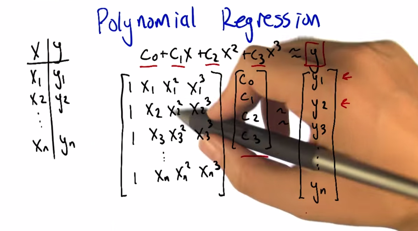
M: Alright. So we talked through how it works when you’ve got you’re trying to fit your data to a constant function, to a zero order polynomial. But let’s, let’s at least talk through how you do this in the more general case. This is, this is what I’ve been doing to, to fit various curves to the data at least implicitly. So, what we’re really trying to do is we’ve got a set of data, x and y. Set n, n examples of x’s and their corresponding y’s. And what we’re trying to find is these coefficients, C0, C1, C2, C3. Let’s say if we’re trying to do cubic regression where C0 gets added to C1 times x, which gets added to C2 times x squared. Which gets added to C3 times X cubed and we’re trying to get that to look a lot like y. Now we’re not going to get to exactly equal y but let’s pretend for a moment that we could. We have a bunch of these examples and we want it to work for all of them. So we can arrange all of the, all these constraints, all these equations into matrix form. If you’re familiar with linear algebra. So the way that we can write this is here are the, here are the coefficients that we’re looking for, the C’s, and here are what we’re going to multiply them by. We’re going to take the X one and look at the zeroth power, the second power, the third power. And that equation I’ll use my hands cause that’s I always, I always need to use my hands when I do matrix multiplication. So you’re going to across here and down there to multiply these and add. And that needs to correspond to y1. And same thing this now the second row. Multiplied by these coefficients. Need to give us our y2 and so forth. Alright. So if we arrange all these x values into a matrix, and we’ll call it, you know, x. And then we have these other guys. And we’ll call this w, like the coefficients. Obviously w stands for coefficient. And we want that to sort of equal This vector of y’s. And we basically just need to solve this equation for the w’s. Now, we can’t exactly solve it because it’s not going to exactly equal, but we can solve it in a least squares sense. So let me just step through the steps for doing that. Alright, so let’s, so here’s how we’re going to solve for w. So what we’re going to do is premultiplied by the transpose of x. Both sides. I mean really what we wanted to do at first is if we are solving for Y, we need to multiply by the inverse of X, but this isn’t really going to be necessarily well behaved. But if we premultiplied by the X transpose then this thing is going to have a nice inverse. So now we can premultiply by that inverse. All right. Now, conveniently because this has a nice inverse, the inverses cancel each other. We get that the weights we’re looking for can be derived by taking the x matrix times its own transpose, inverting that, multiplying by x transpose and then multiplying it by the y. And that gives us exactly the coefficients that we need To have done our polynomial regression. And it just so happens that we have some nice properties in terms of these x transpose x. Not only is it invertible, but it does the right thing in terms of minimizing the least squares. It does it as a projection. Now, we’re not going to go through the process by by which we argue that this is true.

C: Does it have something to do with calculus?

M: It most likely has something to do with calculus. And we’ll get back to calculus later. But in this particular case we can, we’re just using projections and linear algebra. And most importantly the whole process is just we take the data we arrange it into this matrix with whatever sort of powers that we care about. And then we just compute this quantity and we’re good to go.

Errors

scribble

slides

transcript

M: Alright now part of the reason we can’t just solve these kinds of problems by solving a system of linear equations and just being done with it has to do with these squares is because of the presence of errors. The training data that we are given has errors in it. And it’s not that we’re actually modeling a function, but the thing that we’re seeing is the function plus some, you know, some error term on each piece of data. So, I think it’s reasonable to think about where did these errors come from? So, I don’t know, what do you think Charles? Why is it we’re trying to fit data, that has error in it, can’t we just have no errors?

C: I would like to have no errors. Certainly my code has no errors. So let’s see where might errors come from. So they could come from, sensor error, right? Just ,somehow you’re getting inputs and you’re getting outputs and that output’s, being read by, some machine or by a camera or by something and you just, there’s just error in the way that you read the data. Just an error in the sensors.

M: Alright, can you think of other ways. I guess in this case you’re imagining that the data came by actually measuring something, with the machine. So that makes a lot of sense. What other ways can we put together the data?

C: I don’t know I could think of a bunch. I mean the error, well, the errors could come, maliciously. There could be someone out there that is trying to give us bad data.

M: Alright, that seems like a possibility when the data set was collected, let’s say that we’re collecting, various. Oh, this happens a lot. So if you’re trying to collect data from other Computer Science departments and you’re trying to put together, some kind of collection of, you know, how much do you spend on your Graduate students say sometimes these departments will actually misrepresent the data and give you something that is wrong. Because, they don’t want to tell you the truth, because they’re afraid of what you are going to do. So we’re just, you know, we’ve copied everything, but you know, there’s just some of the lines that got filled in just got mistyped. So sensor errors were actually saying there’s something physical, that’s being measured and there’s just noise in that. Transcription error, is similar except it’s a person. Right? The, the there’s a little blips in the person’s head and they can do, it can be a very different kind of error. You can get, like transpositions of digits, maybe instead of um, just you know, noise.

C: Okay, how bout, how bout one more? How about ,uh, there’s really, just noise, in the process. So how about that, that we took in input X, but there’s something else going on in the world, that we weren’t measuring, and so the output might depend on other things besides simply the input that we’re looking at. So what would be an example of that?

M: Let’s look at the housing data. So in the housing data we were just trying to relate, the size of the houses, to the price, but there’s a lot of other things like change of the houses to the price and location. Right those are three really good reasons that are not in the particular regression, that we did that actually influence the prices. So right, the quality of the house and who built it, and, you know, the colors.

C: Even, even time of day, or what the interest rates were that morning versus what people thought they might be the next day. Who knows?

M: Right and so all these different things are being considered in that particular regression, so we’re just kind of imagining that it’s noise, that it’s just having a bumpy influence on the whole process. So what I’d like you to do is select the ones that you think actually are important, the ones that could actually come up, when you’re using machine learning and regression to solve your problems.

M: Alright, and if you know, if you were paying attention as we were going through this, these are all very common and realistic things. So, you know these are all true, these are all sources of error. And this is why we really need to be careful when we fit our data. We don’t want to fit the error itself, we want to just fit the underlying signal. So let’s talk about how we might be able to figure that out. How can we get a handle on what the underlying function really is apart from the errors and the noise that are, that are in it.

Cross Validation

scribble

• Goal to is Generalize.
• The training set and test set are representative of the real world data.
• IID - Independent and Identically Distributed.

slides

We are going to use folds (coming from of folds of sheep) and it will create a model by using one of the folds as test set itself.

transcript

M: Alright, so let me try to get to this concept of cross validation. So, imagine that we’ve got our data, this is our training set. We can, again, picture geometrically in the case of regression. And, ultimately what we’re trying to do is find a way of predicting values and then testing them. So, what we imagine is we do some kind of regression and we might want to fit this too a line. And, you know, the line is good, it kind of captures what’s going on and if we apply this to the testing set, maybe it’s going to do a pretty good job. But, if we are, you know, feeling kind of obsessive compulsive about it we might say well in this particular case we didn’t actually track all the ups and downs of the data. So what can we do in terms of if we, if we fit it with the line and the errors not so great. What else could we switch to Charles?

C: We could just use the test. No, sorry. What, what I mean is if we fit, we fit this to a line and we’re sort of not happy with the fact that the line isn’t fitting all of the points exactly. We might want to use maybe a higher order polynomial. To fit this better. So if we can fit this with a higher order polynomial and maybe it’ll hit all these points much better. You know, so we have this kind of other shape and now it’s doing this, it’s making weird predictions in certain places. So, what was your suggestion? If we trained on the test set, we would do much better on the test set, wouldn’t we?

M: Yes.

C: But that’s definitely cheating.

M: Why is it cheating?

C: Why is it cheating? Well, if we exactly fit the error, the test set. That’s not a function at all, is it? If we exactly fit the test set, then again that’s not going to generalize to how we use it in the real world.

M: So the goal is always to generalize. The test set is just a stand-in for what we don’t know we’re going to see in the future.

C: Yes, very well said. Thank you.

M: Actually that suggests something very important. It suggests that our training set or even if we cheat and use the test set. Actually makes sense unless we believe that somehow the training set and the test set represent the future.

C: Yes, that’s a very good point, that we are assuming that this data is representative of how the system is ultimately going to be used. In fact, there’s an abbreviation that statisticians like to use. That the data, we really count on the data being independent and identically distributed which is to say that all the data that we have collected, it’s all really coming from the same source, so there is no sort of weirdness that the training set looks different from testing set looks different from the world but they are all drawn from the same distribution.

M: So would you call that a fundamental assumption of supervised learning?

C: I don’t know that I’d call it a fundamental of supervised learning per se, but it’s a fundamental assumption in a lot of the algorithms that we run, that’s for sure.

M: Fair enough.

C: There’s definitely people who have looked at, well what happens in real data if these assumptions are violated? Are there algorithms that we can apply that still do reasonable things? But the stuff that we’re talking about? Yes, this is absolutely. A fundamental assumption. Alright, but here’s, here’s where I’m trying to get with this stuff. So what we really would like to do, is that we’d like to use a model that’s complex enough to actually model the structure that’s in the data that we’re training on, but not so complex that it’s matching that so directly that it doesn’t really work well on the test set. But unfortunately we don’t really have the test set to play with because its too much teaching to the test. We need to actually learn the true structure that is going to need to be generalized. So, so how do we find out. How can we, how can we pick a model that is complex enough to model the data while making sure that it hasn’t started to kind of diverge in terms of how it’s going to be applied to the test set. If we don’t have access to the test set, is there something that we can use in the training set that we could have it kind of act like a test set?

M: Well, we could take some of the training data and pretend its a test set and that wouldn’t be cheating because its not really the test set.

C: Excellent. Indeed, right, so there’s nothing magic about the training set all needing to be used to fit the coefficient. It could be that we hold out some of it ,as a kind of make pretend test set, a test test set, a trial test set, a what we’re going to say cross validation set. And it’s going to be a stand in for the actual test data. That we can actually, make use of that doesn’t involve actually using the test data directly which is ultimately going to be cheating. So, this cross validation set is going to be really helpful in figuring out what to do. So. Alright, so here’s how we’re going to do this, this concept of cross validation. We’re going to take our training data, and we’re going to split it into what are called folds. I’m not actually sure why they’re called folds. I don’t know if that’s a sheep reference.

M: Why would it be a sheep reference?

C: I think there’s a sheep-related concept that is called a fold. Like, You know, we’re going to bring you back into the fold.

M: Oh.

C: It’s like the group of sheep. Alright so what we’re going to do is train on the first three folds, and use the fourth one to, to see how we did. Train on the second there and fourth fold and check on the first one. And we’re going to we’re going to try all these different combinations leaving out each fold as a kind of a fake test set. And then average these errors. The goodness of fit. Average them all together, to see how well we’ve done. And, the model class, so like the degree of the polynomial in this case that does the best job, the lowest error, is the one that we’re going to go with. Alright, so if this is a little bit abstract still let me ground this back out in the housing example.

Housing Example Revisited

scribble

• Error increases as we give more power and it sort of overfits the data.

slides

transcript

M: Alright so here’s how we’re going to look at this. So as you may recall, in this housing example. If we look at different degrees of polynomials and how well they fit the data. Let’s look at the training error. The per example training error. So how far off is it for each of the data points? And as we increase the degree of the polynomial from constant to linear to quadratic and all the way up to, when this case order six, the errors always falling. As you go up, you have more ability to fit the data, closer and closer and closer, right? because, each of these models is, is nested inside the other. We can always go back. If the zero fits best and I give you six degrees of freedom, you can still fit the zero. So, that’s what happens with the training error, but now let’s use this idea of cross validation to say what if we split the data up into chunks and have each chunk being predicted by the rest of the data? Train on the rest of the data, predict on the chunk. Repeat that for all the different chunks and average together. So I actually did that. And this is what I got with the cross validation error. So there’s a I don’t know there’s a couple of interesting things to note about this plot. So that we see, we have this red plot that is constantly falling and the blue plot which is the cross validation error starts out a little bit higher than the, the red plot that’s got higher error. So, why do you think that is Charles?

C: Well that makes sense right? because we’re actually training to minimize error. We’re actually trying to minimize error on the training set. So the parts we aren’t looking at, you’re more likely to have some error with. That makes sense if you’d have a little bit more error on the data you haven’t seen.

M: Right, so, good. So in this red curve. We’re actually predicting all the different data points using all of those same data points. So it is using all the data to predict that data. This blue point, which is really only a little bit higher in this case, is using, in this particular case I used all but one of the examples to predict the remaining example. But it doesn’t have that example when it’s doing its fitting. So it’s really predicting on a new example that it hasn’t seen. And so of course you’d expect it to be a little bit worse. In this particular case, the averages are all pretty much the same so there’s not a big difference. But now, let’s, let’s look at what happens as we start to increase the degree, we’ve got the ability to fit this data better and better and in fact, down at you know say, three and four, they’re actually pretty close in terms of their ability to fit these examples. And then what’s great, what’s really interesting is what happens is now we start to give it more, the ability to fit the data closer and closer. And by the time we get up to order six polynomial, even though the error on the training set is really low, the error on this, on this cross validation error, the error that you’re measuring by predicting the examples that you haven’t seen, is really high. And this is beautiful this inverted u, is exactly what you tend to see in these kinds of cases. That the error decreases as you have more power and then it starts to increase as you use too much of that power. Does that make sense to you?

C: It does make sense. The problem is that as we give it more and more power we’re able to fit the data. But as it gets more and more and more power it tends to overfit the training data at the expense of future generalization.

M: Right. So that’s exactly how we referred to this is this sort of idea that if you don’t give yourself enough degrees of freedom, you don’t give yourself a model class that’s powerful enough you will underfit the data. You won’t be able to model what’s actually going on and there’ll be a lot of error. But if you give yourself too much you can overfit the data. You can actually start to model the error and it generalizes very poorly to unseen examples. And somewhere in between is kind of the goldilocks zone. Where we’re not underfitting and we’re not overfitting. We’re fitting just right. And that’s the point that we really want to find. We want to find the model that fits the data without overfitting, and not underfitting.

C: So what was the answer on the, housing exam?

M: Well, so, it seems pretty clear in this, in this plot that it’s somewhere, it’s either three or four. It turns out, if you look at the actual numbers, three and four are really close. But three is a little bit lower. So three is actually the thing that fits it the best. And, in fact, if you look at what four does. It fits the data by more or less zeroing out the quartic term, right? It doesn’t really use this power.

C: Oh, but that’s interesting. So that means it, it barely uses the, the, the extra degree of freedom you give it. But even using it a little bit, it still does worse than generalization.

M: Just a tiny bit worse.

C: That’s actually kind of cool.

Other Input Spaces

scribble

slides

transcript

M: Alright. Up to this point I’ve been talking about regression in the context of a scalar input and continuous output. Sorry. Scalar input and continuous input. So basically this x variable. But the truth of the matter is we could actually have vector inputs as well. So what would might, what might be an example of where we might want to use a vector input?

C: A couple of things. One if you look at the housing example, like we said earlier, there are a bunch of features that we weren’t keeping track off. So we could have added some of those.

M: Great yeah, we could include more input features and therefore combine more things to get it. But how would we do that? So let’s say for example, that we have. Two input variables that we think might be relevant for figuring out housing costs. The size, which we’ve been looking at already, But also let’s say the distance to the nearest zoo. We, we think that that’s a really important thing. People like to live close to the zoo.

C: But probably not too close to the zoo.

M: [LAUGH] Possibly not too close to the zoo. But let’s sort of imagine that the further away from the zoo, you are, the better it is. Just like the bigger the size is, the better it is.

C: Mm-hm.

M: So how do we combine these two variables into one in the context of the kinds of function classes that we’ve been talking about?

C: Well, if you think about lines, we can just generalize the planes and hyper planes. Right so, in the case of a 1 dimensional input. That 1, 1 dimensional input gets mapped to the cost. But in the case of 2 dimensional inputs, like size and distance to the zoo. We have something that’s more like a plane. Combining these two things together in the linear fashion to actually predict what the cost is going to be. So right, this notion of polynomial function generalizes very nicely. All right, there is another kind of input that’s important too, that, let’s think about a slightly different example to help drive the idea home. So let’s imagine we are trying to predict. Credit score, what are some things that we might want to use as features to do that.

M: Do you have a job?

C: I do, actually.

M: [LAUGH] yes.

C: Oh, I am sorry, I am sorry, I misunderstood. So you are asking, you are saying one [UNKNOWN] that could be important for predicting someone’s credit score is just to know do they currently have a job. Right another thing might be well you, you can ask instead how much money they actually, how many assets they have. How much money do they have? Credit cards.

M: Great. So things like, what is the value of the assets that, that they own, right? So this is a continuous quantity like we’ve been talking about. But something like do you have a job, yes or no, is a discrete quantity. And one of the nice things about these kinds of regression approaches that we’ve talking about, like polynomial regression, is that we can actually feed in these discrete variables as well. Certainly if they’re Boolean variables like, do you have a job or not? You can just think of that as being a kind of number that’s just zero or one. No, I don’t have a job. Yes, I have a job. What if it’s something like, you know, how many houses do you own?

C: Hmm.

M: That’s pretty easy because you could just treat that as a scalar type quantity. What about

C: Are you.

M: Type of job.

C: Type of job, I like that. How about hair color?

M: So, yeah, how would we do that? If we, if we’re trying to feed it into some kind of regression type algorithm, it needs to be a number or a vector of numbers, and they can be discrete. So right. So how do we encode this as some kind of a numerical value?

C: Well, we could do something ridiculous like actually write make it kind of continuous.

M: Interesting.

C: That seems insane, but you could do that. Or you could just enumerate them and just assign them values one through six in this case. Right, 1, 2, 6 or they could be vectors like, is it red, yes or no? Is it beige, yes or no? Is it brown, yes or no? Have it be a vector and actually for different kinds of discrete quantities like this it can make it different, right? So in particular if we just gave the numbers. Then it’s kind of signalling to the algorithm that blonde is halfway between brown and black, which doesn’t really make sense. We could reorder these. Actually the RGB idea doesn’t seem so bad to me.

M: Of course, you have an interesting question of what’s the real RGB value. It implies that somehow interpreting between them makes sense.

C: That’s right.

M: It also implies an order right. It implies that the scalar order of RGB is somehow mean something that it’s no different from saying red is one and beige is two. So, if we multiply it, for example, by a positive coefficient then the more RGB you have The better or the worse, right?

C: Hmm. Interesting. Though, in fact what I had in mind here is for RGB, it’s three different hair colors.

M: I thought the g stood for green.

C: There’s, people don’t have green hair, they have gray hair.

M: But I thought the g in RGB stood for green. Yeah it does usually but I’m making a hair joke.

C: Oh oh. I am sorry. I am glad you explained that. You know Michael.

M: No problem sir.

Conclusion

scribble

slides

transcript