Bayesian Inference
Intro
scribble
slides
transcript
M: Hey Charles.
C: Hey Michael.
M: So like I get to lecture near you today.
C: Yes you do. I can even see you.
M: This is, this is crazy. I sort of don’t have my regular pad. This makes me a little uncomfortable.
C: But you look very dashing in your nice blue suit.
M: Thanks. We’re going to record some live action stuff today.
C: Mm.
M: [LAUGH] All right so. Do you remember last time we were talking about Bayesian learning?
C: I do, because I led that.
M: Right. Good point. And so one of the questions that I asked as a follow-up was, these quantities, these probabilistic quantities that we’re working with. Is there’s anything that we need to know about how to represent and reason with them. And you said that I should look into it. Yeah, because I, I just, I yeah you should look into it.
C: So I did. So, and it’s cool. And so I figured it would be fun to tell you about it.
M: Okay, well I look forward to it.
C: Thanks! And also I want to point out, we’re using a different color scheme today. Isn’t that a nice blue?
M: It is a nice blue, its sort of a relaxing blue. As opposed to that blue blue that we used before.
C: It’s like Cerulean… Is it?
M: No.
C: It’s more like periwinkle.
M: No, it’s definitely not periwinkle.
C: Oh you’re right, it’s not periwinkle.
M: Navy.
C: No, it’s too light to be navy.
M: All right, so so good, so right. It turns out that there’s this concept called Bayesian Networks, which is this wonderful representation for representing and manipulating probabilistic quantities over complex spaces. And so it fits in really well with the stuff you were talking about last time.
Joint Distribution
scribble
slides
transcript
M: Alright, so to make this work, we’re going to need to build on this idea of a joint distribution. It’s not going to be obvious right away what this has to do with machine learning, at all. But, I, it’s going to connect. So, just bear with me for a little bit. Alright, so to talk about this concept, what we’re going to do is look at an example. And the example that I think might work, that would be nice and simple, is the notion of storm and lightning. So, here’s a little picture of storm and lightning. And what we’re going to do is say, let’s say, on a random day, at 2 PM. You look outside. And, what I want you to do is say, what fraction of the time, is, is each of these different possible combination of things happening? So, for example, what’s the probability that you look out and there’s a storm and there’s lightning at the same time? So, what do you think?
C: On a random day?
M: Yeah, random day at 2 PM. And we can be in Atlanta since that’s what you’re familiar with.
C: Is it summer? Because that happens more often in the summer.
M: Sure, let’s say summer.
C: It’s fairly high at 2 PM. Let’s say it happens a quarter of the time.
M: Wow, that’s a rainy summer.
C: Mm-hm.
M: Alright. Now, that’s not the only possibility though. It could also be that there’s a storm but no lightning.
C: Right. That happens more often at 2 PM in the summer in Atlanta. Let’s say it’s mm, .4.
M: Wow. Alright. Now what’s the probability that you look at the window and there’s no storm but there is lightning.
C: Maybe 5%.
M: And what’s the probability that you look out and there’s, you know, it’s nice clear there’s no storm no lightning.
C: Coincidentally I picked numbers that made it easier for me to subtract from one. So, it’s 0.3.
M: [LAUGH] Right and so these, there’s only, these are the only four possibilities. We’re saying. And they, so they have to add up to 100%. And so I, yeah it had to be 30 at this point. So, it’s actually more likely that there’s a storm than not, according to what you said.
C: It’s Atlanta in the summer at 2 PM.
M: There you go. Alright. So, this is a joint distribution. And now we can actually ask various kinds of questions about this. Oh, you know what would be a good form for asking a question.
M: I don’t know. I’m looking at you quizzically.
C: Nice. Using the fact that we are in the same place. We are going to do a quiz.
Quiz: Joint Distribution
scribble
slides
transcript
M: You ready for a quiz?
C: Yes, I am.
M: Okay. Here’s what I’d like you to do. I’d like you to use these probabilities that we have written down here, that, that constitute the joint distribution of, when you look out do you see a storm, do you see lightning? And use these numbers to answer some other questions that aren’t directly in here but you can figure it out. So, the first one is to say, what’s the probability when you look out the window at
C: Okay. And, then the question is to say, what’s the probability that if there is a storm, there is also lightning, okay? So the probability of lightning given that there is a storm. And we’ve done some stuff with conditional probability. So these concepts should be familiar with you, but you should be able to connect it up with, you know, the numbers in the table. You ready?
M: I am ready.
C: Go.
Answer
M: All right. Let’s hear it.
C: Okay. So here’s the process that I went through. I’m just going to talk this out. I haven’t actually worked it out in my head yet. So what’s the probability that there isn’t a storm? Well the way you have this drawn it actually makes it pretty easy to see. I can just look at the cases where storm is false, and it turns out there’s two of them. And I can just add those probabilities over there, and I get .05 plus .30, and that gives me .35.
M: That’s great. Yes, so that’s exactly what you did. So you went through, and now all that matters in the universe are the cases where they’re not a storm and that ended up being these two numbers. And you said, well Those are two different cases that can happen. We’ll just add their probabilities because they’re not overlapping and you’ve got .35. Great. All right what about the second question?
C: Okay, so that’s probability that there’s lightning in a world where there’s a storm so I’m going to do a very similar trick. I’m going to look at the cases where storm happens to be true. And conveniently they’re the first two rows and I have two cases, so we know the probability of there being a storm is 0.65 which is good, because 0.65 and 0.35 add up to one. But that’s not the probability of there being lightening, given there is a storm. So, of those two cases, there’s only one where lightning is happening, windstorm is happening, and that’s 0.25. But 0.25 isn’t enough because it’s only 0.25 out of 0.65.
M: Hm.
C: So the correct answer would be 0.25 divided by 0.65. Which is, some number. 5 13th’s?
M: Yeah. It’s 5 13th’s. And, though I’d rather that people fill it in as a fraction.
C: As a, wait. That is a 5 13ths is a fraction.
M: Good point. As a point something something. A decimal.
C: So, 5 13ths is obviously 0.4615. And there you go. Is that right?
M: Yes. That was perfect. Yeah so its usually when there’s a storm, its not lightning. It’s less than half the time. That makes sense.
C: It does because otherwise lightning would be happening all the time.
M: Well when it’s storming. It could be that its very likely when its storming.
C: It is likely when it’s storming, but it wouldn’t be happening every time its storming because otherwise it would be lightning all the time when its storming.
M: Right.
C: And often there’s breaks between lighting. In fact, most of the time there’s not lightning, at least outside my window. At 2pm. In the summer.
Adding Attributes
scribble
slides
transcript
M: Alright, so that wasn’t so bad. You are able to compute some probabilities from this joint distribution. So let’s see what happens when we start talking about more variables. More propositions that could be true or false. What I did is I filled in thunder as another variable and thunder can be true or false in each of these cases. And I wrote down what the probabilities could be from my experience in Atlanta in the summer. I was, I was around over last summer, and in 2004, so let’s, so I’m an expert obviously, so I’m able to estimate these probabilities to the nearest percent. Anyway the point is, that one of the things you should notice here is that each time we add one variable what happens to the number of probabilities that we have to write down?
C: Well in a world where it’s binary it goes up by two.
M: A factor of two, right?
C: A factor of two.
M: Not just, not just two more, but like, twice as many. And so if we have a complicated scenario that we want to be able to reason about, and it’s got, I don’t know, a hundred variables, that’s going to be a lot.
C: That’s, that’s, I can’t even, I can’t even think about that.
M: Yeah, it’s like two to the hundred is.
C: That’s, that’s not even a real number.
M: It’s technically a real number, but it’s an, it’s an unimaginably large number.
C: There’s only like four numbers, one, two, three, many, and too many.
M: So it’s going to be really inconvenient as we start adding more of these and especially if we add variables like, you know, remember the restaurant example that we worked on when we were doing decision trees.
C: Oh yeah those were the days.
M: Then there was variables like food type, and what was the deal with food type?
C: It had lots of values that it could take on.
M: Yeah, yeah like five or something like that.
C: Thai an, American and Italian.
M: Right and so if we had, add variable like that it’s going to multiply the number of probabilities that we need by five. So this is going to get really big really fast. So would it be nice if we had an more convenient way of writing it out in this distribution?
C: Yeah, it would be nice.
M: So it turns out that we can factor it.
C: But I thought we already had a factor of two?
M: Well that was a joke but it actually is pretty close to being the truth, which is the idea that instead of representing all, so, so, in this case, there’s eight numbers. Instead of representing them as eight numbers, we’re going to represent it by you know, 2 times 2 time 2. So we really are going to essentially factor it. putting, putting things into pieces that we can recombine, smaller pieces that we can recombine into, into larger pieces. And it, yeah, it turns out that actually works out really well.
Conditional Independence
scribble
slides
transcript
M: Alright, I’m going to hit you with a definition first.
C: Hit me.
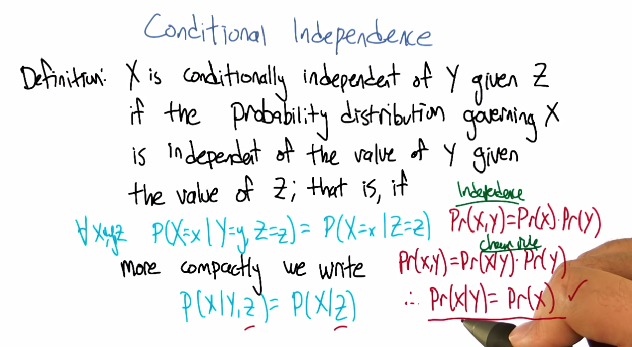
M: So, conditional independence is this idea that goes like this. We’re going to say that some variable that makes up the joint distribution is conditionally independent of some other variable, Y, given Z, if it’s the case of the probability distribution governing X, so the probabilities associated with the values in this variable X Is independent of the value of y given the value of z. So if I tell you what z is, then you can figure out what the probability of x is without having to look at y. So that is, if it’s the case that for all possible values, little x, little y and little z for the variables big x, big y, and big z, If it’s the case that the probability that big X, the random variable big X, equals, takes on the value of little x, given that big Y takes on the value of little y and big Z takes on the value of little z, equals the probability that big X takes on the value of x given big Z takes on the value of z. If those are equal for all possible ways of filling in the values of the variables, then we say that x is conditionally independent of y given z. Right, so you see we dropped Y from the right-hand side of the probability expression. Okay, so it’s sort of less things we have to worry about, if it’s the case that we really didn’t need it in the first place.
C: Fewer.
M: Fair enough.
C: So that’s pretty similar to normal independence. Okay, so what’s normal independence?
M: So normal independence, we say the probability of x and y is equal to the probability of x times the probability of y.
C: That’s right.
M: Which means if we think about the chain rule, we also know that the probability of x and y is equal to the probability of x given y times the probability of y. So that means that the probability of x given y is equal to the probability of x, for all values of x and y.
C: So this is actually implying. So [INAUDIBLE] if it equals that. Oh, that means that px times py equals px given y times py. If we cancel those, we get px equals. Okay. That’s what you wanted to say.
M: Right. So, since, What independence means, right, is that the joint distribution between two variables is equal to the product of their marginals. That’s just. You know comes from basic probability theory and so if you think about what that means from the chainable point of view it’s like saying the probability of x given y is equal to the probability of x. So, it looks just like the equation you wrote down for conditional independence.
C: Right, the only thing that we added is this notion that it might be the case that we don’t have such a strong property as this where it’s always the case that you can write the probability of x given y just with the probability of x. But in the context of some, of knowing some value z, it might be true. And that’s what conditional independence gives us. As long as there is some z that we stick in here, that gives us that property, that’s great, we can essentially ignore why, when we are talking about the probability of x.
M: Okay, that’s pretty cool. That means more powerful or something.
C: Yeah, and in fact if you remember you mentioned the word factoring. You can see here that we are down a probability as the product of two other things. We are factoring that probability distribution. That’s what independence lets us do. And conditional independence let’s us do that in, in more general circumstances. So let’s apply this content back to what we were talking about before.
M: Okay.
Quiz: Conditional
scribble
slides
transcript
M: So, here’s a quiz using this notion of conditional independence. So, bear with me for a second, because this is a little bit weird the way that I wrote it. But, what I’d like you to do is find a truth setting for thunder and lightning. So like, true/true or true/false or false/true or false/false. Such that, the following thing holds true. That the probability that thunder takes on that value, given that lightning takes on the value that you give, and the storm is true, ends up equaling the probability that thunder takes on that value given lightning takes on the value that you gave and storm is false. Right, so a setting here so that basically the value of storm doesn’t matter.
C: So, whatever I put in the upper left box has to be what I put in the lower left box. What I put in the upper right box has to be what I put in the lower right box.
M: Right and in fact we’re just not going to give you boxes for the other ones. We’ll just give you the two top boxes and automatically fill in the bottom box.
C: Okay, that seems reasonable
Answer
M: Alright, so how are we going to figure this out?
C: By you letting them figure it out while I figure it out.
M: I think you should figure this out.
C: Okay let’s figure it out.
M: It might not be obvious just looking at it blankly so why don’t we just throw in some values here. So, for example we can do this.
C: Mm-hm
M: Which is, it gets filled in in both places. So the probability that thunder is true given that lightning is false and storm is true, what is that number?
C: Well, so we just have to find the place in our little eight-row table where lightning is false and storm is true.
M: Lightning is false and storm is true, uh-huh.
C: Which is there.
M: Uh-huh.
C: And the probability that thunder is true is 0.04 divided by thunder is true given that the other two things lightning is false and storm is true so that’s going to be divided by the point 4. That’s the setting that we’re in.
M: Right and Point 04 divided by point 4 is point 1
C: Right so maybe we’ll get lucky and it will work out the same with the other one. So where do we have to look for that one?
M: Well now we have to look in the row where lightning has false and storm is false.
C: Okay. Down here.
M: And look at the case where thunder is true, and that’s .03. .03 divided by .3 which is also .1.
C: Woo hoo! So that works as an answer. It turns out that, in fact, no matter what you type into these two boxes, it does, in fact, work. And what does that tell us?
M: Well, it tells us that it doesn’t matter what the value of storm is. We can figure out the value of thunder by only looking at the value of lightening. So, that is to say, that the probability of thunder given lightning and storm is equal to the probability of thunder given lightening or that we have conditionally independent variables. Yes, that’s right. Storm is conditionally independent of thunder, given lightning.
C: Right. So, the probability of thunder giving li-, given lightning and storm, is equal to the probability of thunder, given lightning. That means that thunder and storm. Are conditionally independent, given lightning.
M: Or thunders conditionally independent of storm, given lightning.
C: Sure.
M: Very good. Alright. So now what we’re going to do next is say, Okay well given that we have this nice property. And yeah, I, I worked a little bit to make sure that the numbers, worked out. It doesn’t always happen this way, but here we had some nice conditional independence and what, we’re going to do next is look at a nice representation of that, kind of information.
Belief Networks
scribble
slides

transcript
M: So the concept of a belief network, sometimes also known as Bayes Net. Sometimes also known as Bayesian Network. Sometimes also known as a graphical model. And there’s other names, but it’s the same idea over and over again. And the, and the idea is that what we’re going to do is we’re going to represent the conditional independence relationships between all the variables in the joint distribution graphically. In terms of of a little picture like this, where there’s nodes corresponding to all the variables. And, edges corresponding to dependencies that need to be explicitly represented. So, the way that this works is, what we can do is we can fill in the prior probability of storm, which we can get by just marginalizing out. So we’ve, we’ve already done an exercise like this. So this is a number you should be able to figure out. Then because of vary well, this is also true that that you can figure out what the probability of lightning is, given storm and also given not storm. And these are numbers that you can just get by marginalizing out. Finally, the probability of thunder, normally you’d have to condition that on both storm and lightning. But as we already talked about, it’s actually conditionally independent of storm given lightning. So, all we need to figure out is the probability of thunder given lightning, and the probability of thunder given not lightning. And once we have these, in this case five numbers, that’s enough to work out any probability we want in the joint, just by multiplying corresponding components together. So, what I’d like you to do is actually fill in these boxes as a quiz. And to help you out we copied the numbers over from the previous slides so that you actually have the values that you need to fill in this table. because otherwise that would have been kind of mean.
Quiz: Belief Networks
scribble
- Statistical Independence
slides

transcript
M: Hey Charles can you work out these numbers?
C: I can. So the first one is pretty easy because we did that once when we were talking a couple slides back.
M: We did.
C: We just look at the case where a storm is set to be true. Those are, those two mega rows there and those are .25 and .4. We add that up and we get .65. We’re pointing out that since we know that S is .65, we know that not S is .35.
M: Good.
C: Okay. Although that table really has two numbers in it, we only need one of them.
M: Right. Yes. Very good point.
C: because it’s constrained by needing to add up to one. Then we do something similar with lightning. We look at the cases where lightning is true. And s is also true.
M: Yep. There’s just one case like that. Huh?
C: Huh, there is only one case like that.
M: Right, but what we really want to know is what’s the probability that lightning is true given that storm is true. So we need to think about both cases where storm is true and say of these, what’s the probability that storm…that lightning is true.
C: And it’s .25 over .65.
M: Right.
C: Which is .385 rounded up.
M: because you’re a cowboy.
C: Which means that… The probability of it, of not L given S is one minus that or .615.
M: That’s right.
C: Okay. So we do the same trick with probability of L given not S and we find the case where lightning is true but storm is false and that’s .05, or we have to do it out of both cases where S is false and so it’s .05. Divided by, point .05 divided by .35 which is, 1 7th. And 1 7th is approximately .143, rounded up. And so not L given not S is .857.
M: [LAUGH] Nicely done.
C: I use subtraction in my head.
M: In your head yeah, but it was like with caries and stuff that was nice. And right, so let’s see. And, does these sorts of things make sense. Of not a storm, it’s kind of unlikely that we’ll see lightening. Or, if there is a storm, it’s moderately common that we’ll see lightening.
C: Okay, that makes sense. Okay, good. So, now we do the same trick again with thunder. Except now, instead of looking at l n s, we look at > Thunder and, and lighting, so we need to look a case where thunder is true and lightning is true, so that would be, point, that’s all the cases where lightning is true, so it would be .2 divided by .25
M: Alright and why are we looking at the case where storm is true?
C: Why are we doing it? Because it’s conditionally independent of storm.
M: It doesn’t matter.
C: [CROSSTALK] Information, so it doesn’t matter which rows we look at. What matters is we look at a case where thunder and lightening are both true, and we compare that to thunder is false and lightening is true. So that’s this number. Those add up to the 0.25, we get 0.2, over the 0.25, which is 0.8. Right.
M: So it’s very likely to hear thunder if you see lightning.
C: That makes sense. And there’s only a 20% chance that you don’t hear thunder when you hear lightning.
M: It’s lightning not thunder, yup. Mmhmm.
C: And so we do the same thing in the case where we have thunder and there’s not lightning. So we find that row.
M: Okay. Not lightning and there is thunder. There’s one.
C: Right and we do the same trick we did before and we get, .04 over .4. Which I think we did last time, actually, and we get .1.
M: We did. So, if it’s, if there’s not lightening out, it’s very unlikely to hear thunder. Alright.
C: Alright and just to drive this point home. That was great. Just to drive this point home. What if it was the case that it mattered what’s value storm had, how would we fill in this table.
M: Well we’d have to look at a lot more rows.
C: Well in particular we couldn’t draw this kind of leaf network if that were the case, right?
M: Right.
C: Because it wouldn’t be conditionally independent. So we’d have to draw basically another edge. Here, and what that represents is that thunder, to work out to what the proper? of thunder is, you have to look at storm and lightning, all the joint combinations of those to make it work.
M: And that grows exponentially as you add more and more data. << And that’s right, and that’s something that threw me when I started to look at this, because the picture looks a lot like a neural net. Right? In a neural net, you’ve got these nodes, you’ve got arrows going into the nodes, and when you have a bunch of arrows going into the same node, you just end up like adding all those different influences together, weighted by what’s, what it has on the weight. This belief network representation is an entirely different animal. In particular, now, what we’re really saying is, to work out the value of this node, you need to know what’s going on in all combinations of what the inputs are. And so, as you pointed out, so astutely, that grows exponentially as you have more variables coming into the node. Higher in degree.
C: Hm. So this is not just a network. It’s a graph. And so we can talk about parents and children right? So, basically, the number of numbers you have to keep track of is exponential in your number in your parents.
M: I mean it’s a, yes. Though it’s not exactly a tree. Doesn’t have to be a tree so the parents relationships are kind of weird. Like in particular, if you use parent terminology in this graph, what you’re saying is that lightning has one parent which is storm and thunder has two parents which are storm and lightning. So it’s, storm is it’s own grandfather and parent.
C: So let me ask you a quick question, Michael. So earlier on when you were describing this, this graph, I noticed you used the word dependencies. You said we’re going to capture the dependencies.
M: Hm.
C: So if you erase the red line between storm and thunder,
M: I’d be happy to.
C: So you erased that, should I read this as storms cause lightning, and lightning causes thunder.
M: You can do that, but you would be wrong.
C: Oh okay.
M: You can not infer that there is a cause of relationship just because there is an arrow between them. These arrows are just telling us about the relationship between the probabilities and not anything about the physically processes that underlie them.
C: Okay so let me make sure I understand, what you are saying is, it would be very natural to look at a belief network or a [UNKNOWN] net or a Bayes Nets or graphical model. And read the arrows as causes, and therefore read them as talking about dependencies. But actually what’s happening here is that these things represent conditional independencies. So, it is not true that lightning is dependent on storm and thunder is dependent on lightning. So much as is the case that storm and thunder are conditionally independent given lightning.
M: That’s, that is a good point. I guess I never really realized that dependence. You use the word dependence. Sometimes it means a physical dependence. Like, in the real world it’s dependent. Here I’m just talking about statistical dependence. It’s really just talking about the fact that we can derive numbers from other numbers, and not that You know things cause other things. So yeah, that’s a really good point. It seems like that was an easy place to get slipped up.
C: Okay. Cool.
Quiz: Sampling From The Joint Distribution
scribble
slides

transcript
M: Alright, so now that we have a handle on this kind of representation, let’s look at some things we can do with it. So, here’s an example of a Bayesian network with five variables. A, B, C, D, E. And let’s pretend that each one has some set of possible values. Could be true/false. Could be red, green, blue. Whatever it happens to be. And these arrows again tell us about our conditional dependence relationships. So how would we go about actually well, say sampling from this distribution? So let’s say that we wanted to just as an example see what A, B, C, D, and E, might look like in a, in a randomly selected example from the distribution that this network represents. So turns out what we can do is that if we sample from A. Now A is specified has no incoming arrows so it’s not conditioned on anything in particular so we can sample directly from A’s distribution. We can do the same for B and now C. If we want to sample from C, we need to, make use of what values have already been selected for A and B. Because C is conditioned on A and B. But we can sample from that distribution. Each, each value of A and B, each joint value of A and B gives a distribution over
C. And we do the same thing for D and the same thing for E. And we’re done. What we’ve sampled from is actually the probability distribution, the joint probability distribution. So does that seem like a useful thing to be able to do Charles?
C: It does seem like a useful thing to be able to do.
M: Yeah, so here’s just a quickie quiz. So just write a one word description that says, well in this sampling you’ll notice I went a, b, c, d, and e. What ordering do I need to do if I have a belief net like this specified by this graphical structure with the arrows? If I want to be able to sample it, I need to do it in a particular order. Some orders are, are going to be problematic because we haven’t actually, you know, sampled the variables that it depends on. So, what ordering should we select for A, B, C, D, E? In general, what, what is the name for that. So that we can actually do this kind of sampling trick this way.
C: Okay.
answer
M: All right Charles, so, so, what do you think the answer is here?
C: Actually I don’t know what you’re looking for here.
M: Oh, okay. Well, so one thing that’s true. We had to sample the, the variables from A to E.
C: Mm-hm.
M: And that’s alphabetical order. So do you think that’s what I was looking for?
C: Maybe in this case but I would think that that wouldn’t be generally true.
M: True. Right. So, yeah, alphabetical is not what I was looking for. So, there’s it’s a graph theoretic property that says we want to basically put the nodes in order, so that you always put the things that have incoming links that haven’t been visited yet after the ones where you, they have been visited.
C: Oh, so it is a lot like alphabetical or a lot like lexo-, lexicographic, but it’s topological.
M: There we go. Yeah, that’s what I was looking for. So, topological sort.
C: Which makes perfect sense.
M: Right, and so this a standard thing that you can do with a graph, and it’s very quick to, to actually compute one of these. It does depend on a particular property, though.
C: Let’s see. Topological only makes sense if you really can go from no parents to parents. So, it cannot be cyclical. You can’t have arrows that take you back. So, E can’t be a parent of A and also have A be one of its parents.
M: That’s right.
C: So it must be acyclic.
M: Must be acyclic, right. And that’s going to be true in these cases, because we’re always going to set it up so that in a, in a Bayes net, the variable that we’re each variable depends on other variables. But they all, it ultimately has to bottom out. There can’t by cyclic dependencies. So, it is a directed acyclic graph.
C: So, what would it mean if there were cycles?
M: I don’t know. I don’t know what to do with such a graph.
C: It just doesn’t mean anything at all, I guess.
M: Yeah, I mean, there, there is a family of undirected models.
C: Mm-hm.
M: But we’re talking only about the directed ones here. So, the directed ones yeah, it’d have to be acyclic for the, for the probability distribution to be meaningful.
C: Well, that makes sense.
M: I’m sure we could make something up, but this is, typically this is how it’s done. It’s, it’s, we constrain ourselves to acyclic graphs.
C: Well, if a Bayesian network is supposed to capture conditional independencies, then if you add cycles, that’s like saying there are none, right? I’m not even sure what that means.
M: I could make it mean something. So here, we, we want the probability of A, conditioned on probability of A. Well, maybe that’s like probability of what, what A was one time step ago. Or it could mean that it, you know, that, that we’ve actually putting constraints on the joint assignment to all the variables. But, yeah, it’s not really, it doesn’t really, it makes things more complicated and that’s not the model that, that is the typical one
C: Okay, fair enough.
Recovering the Joint Distribution
scribble
slides

transcript
M: So another important thing that you can do with this representation is recover the joint distribution. Remember a couple, a couple slides ago we looked at the issue of how can we go from the distrib, joint distribution to specifying what the probabilities are, the conditional probability tables, they’re called, at each of these nodes. But we can actually go the other direction as well. We can go from, from the values in these conditional probabilities tables in each of the nodes, to computing the probability of any combination, any joint combination of variables that we want. So, it turns out it’s really, really simple. We can just go and use these same ideas and say the joint probability for some assignment to the variables, is equal to just the product of all the individual values. So the probability that that value of A would be taken times the probability that that value of B would be taken times the probability that that value of C would be taken, conditioned on those are the values that were chosen for A and B. So it’s just like in the sampling case.
C: Right, and that’s much more compact a representation.
M: That’s a good observation, yeah. So how, if these were Boolean variables, how many values would we need to specify for the joint distribution in the standard representation, where you just assign probability to everything.
C: Well if I ignore the fact that there are some constraints that we might be able to take advantage of, it would be
M: Right, but here we’ve broken it down into smaller chunks so, the probability of A, it’s just specified by single number. Probability of B is specified by a single number. Probability of C is specified for a single number for each combination of A and B. That’s four of them. This also requires four values and this requires four values. So this is really, what, it’s like 2 to the 5th minus 1 I guess. Because, if I tell you the first 31 values, the last, the This is 14 numbers versus 31. You are right, it is more compact, 31 is bigger.
C: Right but let’s imagine that all of the variables were in fact completely independent of one another, then you would have 5, you would only need
M: Yeah, which is what we’d get if we had kind of like just a set of weighted coins. If they’re unrelated to each other, but each one has some probability of coming up heads, the probability of getting some, some particular combination like, A is heads and B is tails and C is heads and D is heads and E is heads. We could just break that down to the probability of the individual events.
C: So then all of the, just like with the joint distribution where you have this exponential growth, because you need to know everything. Here you have the exponential growth that only depends upon the number of parents you have. If you have no parents, then it is constant, if you have parents, then is grows exponentially with the number of parents.
M: Right, so the fewer number of parents, the more compact the distribution ends up being.
Sampling
scribble
slides

transcript
M: Earlier I mentioned sampling and I asked you whether that sounded useful, and you said it was. So, let’s do a little exercise. Why? Why [LAUGH] is that a useful thing? Why is it good idea to be able to sample from a distribution?
C: Well, because it’s one of the two things that distributions are for.
M: What does that mean?
C: Well so why do you have a distribution? A distribution is so that given some value, you can, you can tell me what’s the probability of me seeing that value which is kind of what it looks like when you have the probability function, but also if you have a nice distribution you can generate values according to that distribution.
M: Okay. That’s a little bit circular in the sense that it didn’t tell me why it was useful to generate them other than it’s one of the things you can do.
C: Well, you didn’t ask me to actually make sense. But I mean, this is the, the thing that you use distributions for. Now why would you want to do that?
M: Yeah.
C: So, if a distribution represents kind of a process, it would be nice if I could duplicate that process, right? So, I would have to be able to generate values in the right way, consistent with the distribution in order to generate that process. So it’s like flipping a coin, or I want to flip a coin and find out whether I’m going to get heads or tails. It would be nice if I can do that in a way that’s consistent with whatever the underlying bias of the coin is. M: Okay, so yeah, if this distribution represented something complex, we might, you know, for whatever reason need to simulate that world and, and act according to those probabilities. So, yeah, that, that’s a reasonable one. What else, what if, what if I showed you this, if i took this distribution that we used for the lightning and thunder example.
C: Mm-hm.
M: What if you wanted to get a handle on it? How can we use sampling for the distribution to give you some insight into how the storms work?
C: Okay so let’s see, I’ve, I’ve, I’ve got this representation of the joint distribution, but it’s just a representation of the joint distribution. If I want to asked a question like, well what’s the chance that it’s, oh let’s say, storming outside if I’ve heard thunder, I could go through and, and, you know, back compute the reverse of the conditional probability tables. And I could do things like, or I could just generate a bunch of samples where I had thunder and I can just see how often the storm was also true. Does that make sense?
M: It does, though I’m not going to use the words that you just used to write that down.
C: Okay.
M: I’m going to call that approximate inference. So the basic idea is that you would like to do some inference, you’d like to figure out what might be true of the world in different situations. Instead of doing some complex probability calculation, you’re just going to imagine a bunch of possible worlds and see how often is it the case that whatever it is you want to figure out is true. So yeah, that, that turns out to be a really good way to do it. In fact, sometimes I think that’s a lot of what people are doing when we’re, when we’re making judgments in the world. We’re just really, really good at this kind of sampling from past realities that are relevant, and we can make judgments based on that.
C: Hm. So, how would you do that?
M: How would I do what?
C: How would you do this approximate inference?
M: We’re going to get to that but I wanted to.
C: Oh, okay, cool.
M:But there, but there’s one or two other things about sampling that I wanted to mention.
C: Okay.
M: Another thing that I could imagine using this for is this notion of visualization. Which may be, I mean this in a, in a broader way than it sounds, not necessarily to actually see what the distribution is like, but to kind of get a feel for it. So, I bet if I was to run that if I was to draw a bunch of samples from the lightning thundering set, you would have a better feel for how likely different things are. Just you as a person might get a sense of how these things work. So, you can imagine in, in a medical domain a doctor who’s, who’s thinking about prescribe, prescribing a particular kind of drug for a particular kind of person, if the information about drug interactions and so forth was, was represented as a big belief net, it might be hard to look at it and know anything. But if you use that to generate a bunch of artificial patients you might start to get to feel for oh, you know what, these kinds of people tend to react badly in these kinds of circumstances.
C: That’s still a kind of approximate inference, right?
M: That’s right. So this is, this is a kind of an in the machine sense, and this is kind of in the human sense.
C: Okay, I like that. So let’s see, let’s see if I, if I understand this. So the, the nice thing about the storm, the thunder, and the lightning example is that it has pedagogical value. Because it’s easy for a student to look at that and go okay, I understand what’s going on here. One because there’s only three nodes and two arrows, and the other is because, we think we understand how storms, thunder and lightning work. Right.
M: Yup.
C: Or most people do. So that makes a lot of sense. Of course the downside of it is, we think we understand it. And so it’s hard to see why you would need to do samples, I mean, there’s just a couple of probability distributions and we kind of know what it means. But in the real world, there are perhaps hundreds and hundreds of variables with complicated relationships and conditional independencies that, that aren’t necessary intuitive just by looking at the graph. And so picking one conditional probability table and looking at it isn’t going to tell you much. But by sampling I get real examples that are concrete that, as a human being, I can understand without having to, you know, really glock all the 25 different conditional probability tables. Does that sound right? Is that.
M: Yeah, yeah.
C: What you’re trying to say?
M: That’s exactly right. Thanks.
C: Okay.
M: I want to draw your attention to this, this word here for a moment. This notion of approximate inference. Now generally we don’t like approximations when we can do things, things exactly. So why are, why are we not doing things exactly?
C: because it’s hard.
M: It’s hard, that’s exactly right. So or, or, even if it weren’t hard, it may, it may be in some cases faster. So I would be, I’m not going to do it now, but I’d be happy if I guess if there’s ground swell of support among the students. To I can go through the argument as to why this inference is hard. There’s a nice little reduction to problems, N, NP complete problems like satisfiability. But it turns out roughly that if you could do inference exactly on any belief net that you want, then you could solve very, very hard problems efficiently using that idea. So it’s, it’s cute, but it’s kind of takes us a little bit off our path, so I’m not going to get into that.
C: Okay, so sampling is useful, Michael, which I always suspected in my heart, and now we’ve got some good arguments for why it actually is.
Inferencing Rules
scribble
slides

transcript
M: So, okay so let’s, let’s actually do some inferencing just to, to kind of get a feel for it. For certain kinds of networks we can do things exactly. And we’re going to look at one of those examples in just a moment. But, it turns out, helpful to remind ourselves of some rules of probability in inference that will help us do that. So, here’s just kind of a little cheat sheet. For you, so, marginalization is this idea that we can represent the probability of, of a value, at, by summing over some other variable and looking at the joint probabilities of those. And if, if you’ve trouble remembering this one, this, this’s how I like to think about it, if we’re trying to figure out the probability of x, then one way, one thing we can do is break it up in. Break the world up into, well the cases where x and, not y. Plus, places where x and y. So, the probability of x is it can be broken down into the probability of x when y is false plus the probability of x when y is true. So it’s really simple in that sense, but it actually turns out to be a useful thing to be able to do. To marginalize out. The chain rule, we’ve used this a bunch of times. The probability of x and y can be written as the probability of x times the probability of y given x. And that’s important that we’ve the given X. If we drop that then what is that implying? Just go ahead.
C: Well, if you drop that then it implies that they are completely independent of one another.
M: Right, in the case where the variables are independent, you can just look at their product. In the general case you actually have to look at the second one given the first one.
C: And as I recall, the order on the left doesn’t matter, so, you’ve the probability of X times the probability of Y, but you could have written the probability of Y times the probability of, X given Y.
M: Yes. And, actually, let’s do a quick quiz.
C: Okay.
Quiz: Inferencing Rules
scribble
slides

transcript
M: All right. So, person who’s adept at manipulating Bayes Nets would know that this chain rule idea, this probability of X and Y can be written either as a probability of X times the probability of Y given X. Or as the probability of Y times the probability of X given Y, actually correspond to two different networks. So which of these two networks corresponds to the fact that the probability of x and y, the joint probability of X and can be written as the probability of Y times the probability of X given Y.
C: Go
Answer
M: Did you get it?
C: Yeah I did actually. so, so this one I think I understand completely. So we know that from the last discussion we had about how you would recover the joint, that what you’re saying on the right of this equation probability y times probability n y means that the probability of y, the variable y doesn’t depend on anything. So, between those two graphs the one on the right is the one where you’re saying that. You don’t need to know the value of any other variable in order to determine the probability of y.
M: Good.
C: So it has to be the one on the sec, the second and just to make sure if you look at the second product the probability of x given y the second multican? Is it multican?
M: Hm, factor.
C: Factor? Let’s say factor. The second factor, this says that while you determine the probability of x given the value of y and there is an arrow from y to x so, the second one is in fact correct.
M: Yeah. So this is actually just one way you could just read this network is to say what is this node x with an arrow coming into it? That is the probability of x. But, the, the things pointing into it are what’s exactly being given. What it’s being conditioned on. So that’s exactly right, the second one.
C: Right. So this, this, so this makes sense to me. This is why when you look at a network, network, it’s very hard not to think of them as dependencies. Even though they’re not dependencies, they’re conditional independencies.
M: Well the arrows are a form of dependence but it’s not a causal dependence necessarily, it’s it’s again it’s just the way the probabilities are being decomposed.
C: Hm.
M: And the last of these three equations just Baye’s rule, this time written correctly where the denominator has to be the probability of x, and we’ve gone over this a couple of times. I don’t, I don’t need to, to describe it again, but what Would like to, just, bring to your attention to this three together turn out to be kind of our, you know, three musketeers in working out the probability of various kinds of events.
C: Excellent.
Quiz: Inference by Hand.
scribble
- Very interesting.
slides

transcript
M: All right. So let’s put some of these rules into play by actually doing some inference by hand. Ultimately, we’re going to derive some algorithms that can do this so you don’t have to think about it so hard. But understanding those algorithms, it’s helpful to have gone through an exercise where you actually use these ideas. So here’s a setup. Let’s imagine that we’ve got two boxes. Onee has 4 balls in it and one has 5 balls in it. And we’re going to choose one of those boxes uniformly at random. Either the box that we choose is equal to box 1, or the box that we choose is equal to box 2. And after that, we’re going to draw at random, uniformly at random, from what’s inside the box, one of the balls, and let’s say it turns out to be green. All right. So the draw that we make, we have a green ball. We reach into that same box a second time, and the question is, what’s the probability that that second ball will be blue, given that the first one we drew was green? So let’s, to make, maybe to help point out how this is connected with Bayes net inference, Charles, why don’t you help me draw the Bayes net that corresponds to this problem.
C: Okay. So, if I think about it as a process, which now means I’m, I’m thinking about this as things causing the other, the first thing that you did in the process is you picked the box.
M: Good. All right. So let’s say, so the first variable in the net is going to be the box variable.,
C: Right, and then once I had the box variable over there, I can then pick, the second thing in the process is I pick a ball. So, in this case you’re calling it 1. So I make the first pick.
M: And is it, do we need an arrow there?
C: Yeah, because the, you pick the box and then that let’s you pick which ball that you have. So, which ball you pick, the color of the ball you pick, depends upon the box so to speak.
M: Good. And so, the probabilities here are going to be, it’s going to look like this. All right. So the second variable here is what, what color ball you get when you do the first draw from the box. Ad we can represent this as a conditional probability table. So for box 1, it’s three quarters green, one quarter yellow or orange, zero for blue. And for box 2, it’s two fifths, zero, and three fifths. And so that captures what happens on the first draw.
C: So for the second draw, well, clearly, that sort of depends upon what you drew the first time. Because you said we were drawing without replacement. So it definitely depends upon what you, what you drew the first time. But also, it still depends upon the box. Okay, so now we’ve got tables for a box, we’ve got tables for ball 1, and we need to know what ball 2 is going to be. Well, the value that ball 2 takes definitely depends upon whatever value ball 1 takes.
M: Sure.
C: But it also depends upon which box you’re in. So you need an arrow from there as well. And what would be really nice is if we were in the storm, lightening and thunder case where, if I knew that it was, what ball 1 was, I would know what ball 2 was, but that’s not true. Because in a case, for example, when ball is unless I also know which box I’m in. So, we have to draw the arrow from box to ball 2.
M: Indeed. Right. And so there’s a lot of, a lot of probabilities that we have to write down. But lets, let’s just write down a piece of that table. Let’s say that the value of ball 2 depends on which box. And it depends on what ball 1 is. But let’s just look at the piece of that table where ball 1 is green.
C: hm.
M: because that’s what we’re ultimately going to need here. So now ball 2, in the case where we were drawing from box 1, that probably that’s green. In the case were the first ball had been green, it leaves just 2 out of 3, right.
C: hmm.
M: And 1 out of 3 yellow and no blue. But on the other hand, had we drawn from box 2 first, and again, we had gotten green, now it’s green one fourth, zero yellow, and blue three quarters.
C: RIght.
M: And there’s yeah, we need this same thing where the other case, where ball 1 is yellow and ball 1 is blue. But we are not going to need those numbers for this problem.
C: Right.
M: All right. So now that we have written it as a Bayes net, is that, is that helpful at all? So what we’re, we haven’t asked the question yet. So maybe it’s time to ask the question and then we could work on the answer.
C: Okay.
M: All right. The question is, what’s the probability that the second draw is blue, given that the first draw had been green? Go.
Answer
M: All right, so can you use this Bayes net to help work things out?
C: Yeah, actually it make it a lot easier. I was, I was thinking about how I would do this and, and wouldn’t involve writing a whole lot of equations and doing a whole lot of stuff but actually, just by writing out the Bayes net we ended up, and filling out these tables we ended up doing that. So, the, the bottom table is, basically tells me the probability of, ball two being some color. In a world where ball one is known to be green. Because we just broke down that part of the table, so we don’t have to do it for every other one. And, you know, if I knew that I were in box one, then the probability of it being blue in a world where ball one was green is in fact zero. And if I knew I were in box two. Then the probability of it being blue in, where ball one is green, and where box two is three quarters. So I only care about that last column.
M: All right.
C: And now I just have to choose the row or choose how to distribute the likelihood over the row. So all I really need to know is, what’s the probability of me being in box one and being in box two.
kM: All right, which we have in the table as well, as a half.
C: Right. So that means the probability of it being ball two. Being, ball two being blue in a world where ball one is green, is just the probability of ball two being blue, given that ball one is green. And we want to know the probability two is blue given that one is green but when you look at the table and all we care about is that last column, all we really want to know is, well, we know the answer when box one, when we’re in box one, when box equals one, it’s zero, and we know the answer when box equals two, it’s 3 4s. So if we were going to do a sample, for example, which we talked about earlier, we would just sample a bunch of times, and we would get be great, except of course, we want to compute this exactly. And we know how to compute it exactly, because we actually know the distribution over, how many times box would be equal to 1 and how many times box would be equal to 2. It would be half in each case. So, I really like, I think you’ve made this easier by giving us the table. So, actually writing out the Bayes net. So we want to know the probability that the second ball is blue given that the first ball is green. And that’s just equal to the probability that the second ball is blue. Given that the first ball is green and we were in box one. Because if we knew that, we knew we were in box one and the first ball we drew was green, it’d be really easy to compute the probability of the second ball being blue. It’s right there in the table at zero.
M: Is this, is this the way that you think it should be written?
C: Almost, but not quite. That would be the easy thing to do because we know that answer. We know the probably that box is equal to 1. It’s just a half. But it’s not just the probability that box is equal to one, it’s the probability that box is equal to one in a world where we knew the first thing we drew was green.
M: Gotcha.
C: And if we had that then it would be easy to figure out the, the products there to figure out two is blue in a world where the box one is green. Boxes equal to 1 and the first ball that we pulled was equal to, was green. And then we will just add that to the probability that the second ball we drew was blue. Given that the first ball that we drew was green. And we were in box two. We were drawing from box two. And that would have to be weighted by the prober-, probability that box was two in a world where the first ball that we grew, drew was green.
M: Good. Very good. And in fact, this rule that you kind of worked through follows just algebraically from two of the rules that we just talked about. It’s the combination of the marginalization rule, which lets us introduce this box variable. But the way that we wrote it before, it was, you have to and it in. But then we actually then applied the chain rule to split that into a conditional probability. So, so this is all valid at the moment. And are these quantities that we, that we know?
C: Well, we certainly know the very first term in each of the two summands. Can it be summands? Let’s say they’re summands. If they’re not, we’ll get nasty emails from people. The first part’s probability. Second ball is blue given that the first one is green in red box one. And the probability that the second ball is blue given that the first one is green in red box two. That’s easy, that’s actually in the table.
M: That’s easy, that’s in the table. And it’s zero in this case, and three quarters in this case.
C: Right, so it’s zero in the first case and it’s three quarters in the second case, straight outta the table. Now all we have to do is figure out how often we’re in box one and how often we’re in box two and if you didn’t think it through you would just have the probability of box equals one and the probability of box equals two. But we have to remember we’re in a world where the first ball we picked was green. So now we just have to compute each of those terms. So how do we do that? So we want to know what the probability is that boxes, we’re in box 1 given that we picked a green ball first. Well that one’s actually much easier to think about because Bayes’ rule will give us, will allows us to express this in quantities where we do know the answer. Because we have the tables. So that would be the probability that the first ball was green given that we were in box 1 times the probability that we’re in box 1 divided by the probability that the first thing we picked is green. So, the probability that we get a green ball if we pick box one, is just well, it’s three quarters.
M: Yep. It’s.
C: A different three quarters than the other one though.
M: Yeah. Those, those two three quarters aren’t the same three quarters. This, this way. Because sometimes, two three quarters are not the same two three quarters.
C: In this case, there are three green balls and one, what we’re pretending to call yellow because it’s easier to write than orange, ball. And so three of the four of them are green, so if we were in box one, we close our eyes, we’d get three of those. So what the probability that we’re in box one? Well, it’s right there in the table, to Bayes’ net, it’s one half. Now we just have to figure out well, what’s the probability that I would get a green ball the first time I picked one?
M: Right. And so one easy way to do that is, we actually do this, this whole process again on box two, and then just normalize. Or we could break this apart using the, using the marginalization rule.
C: Yeah, which one do you want to do?
M: The first one I think.
C: Okay. So figuring out the probability the first one is green isn’t, isn’t as easy as it looks. You can’t just say, well there are five green balls, but there’s a total of nine balls, and so it’s 5 9th, because those nine balls aren’t distributed equally on both sides of the boxes. So you really have to, you still have to know which box that you’re in, in some sense.
M: Right.
C: But we can kind of skip that step. Okay, so I like this, so what’s the probability that the first ball is green given that we’re in box two, well it’s just 2 that we’re in box two? Well, it’s just a half because that was given to us on the table. And so, we still don’t know the prior probability of, of the first ball being green, but it turns out we don’t have to because there are only two boxes and so we can just normalize and the right thing will happen. So, three quarters times one half is equal to three eighths. And 2/5 times that’s right. So 3/8 is also 15 over 40. 1/5 is 8 over 40. Why do we do that? Because we want to be able to add them up and normalize and so that means if you added those two together and put them in the denominator, that would give you 23 over 40. And, so how much is 15 40ths of 23 over 40ths well, it’s 15 out of 23. And so, without ever directly computing the probability that us being in box 1, given that the first ball pulled was green is 15 over 23. Which was a lot of work to do considering that we knew we were going to multiply it by zero.
M: [LAUGH]
C: Which meant none of this work mattered.
M: Okay.
C: Or we did it because we love probability.
M: No it was, it was kind of helpful because we needed to know how to normalize these two numbers.
C: Right, so it was useful but, I mean, just the whole thing we already kind of knew.
M: Yeah.
C: That [LAUGH] that was going to be zero.
M: But this one we didn’t know.
C: Right, this one we didn’t know, and so now we know that the, the other case is 8 23rds, and we’re done. So 0 times 15, divided by 23 is
M: Right, and we can, there’s a factor of
C: That’s what I said.
M: Woohoo!
C: Wow.
M: [LAUGH] Boy it would be nice if we had an algorithm to do this for us.
C: Man, and the algorithm shou, shou, should not involve me. [LAUGH]
Naive Bayes
scribble
slides

transcript
M: Alright, so what we’d like to do is work up to an algorithm that can actually do some of these inference steps instead of having to think it through each time de novo. So what I’m going to do is, let’s hearken back to an example that we looked at before which is about spam detection. Do you, do you remember the spam example?
C: I do remember the spam example. That was way back in the boosting lecture, right?
M: Yes, I think you did that one. I did, it was an excellent example.
C: There you go. So, we didn’t think about it in a Bayes net setting, it was in a classification setting we were trying to come up with the rule, but let’s think of this as a Bayes Net where there’s a bunch of different variables that can be true or false about any given email message. It can either be spam or not. It can contain the word Viagra or not. It can contain the word prince or not. It maybe contains the word udacity, or not.
M: Mm.
C: Right? And, so, just as we think about these as these random variables. If we’re trying to build a belief net or a base net with these variables. We have to say. kind of, what’s dependent on what. In terms of representing the probabilities. So how would you, how do you think we should draw arrows to,to relate these to quantities to each other.
M: I think that the arrows should go down from spam to the other features of spam mail and I’ll tell you why. Because if, I like this notion of generation that you talked about a little bit earlier. It seems to me if you know. Spam mail or not. It sort of generates certain words. And as written as these are like words I mean I know the, the spam example these are you know, kind of stand ins for features. But they’re sort of features of spam mail. Yeah I think that’s a really good way to think about it. So, in some sense what we’re saying if we draw the bayes net in this way, then any given email message has some probability of being spam. And given that it’s spam, it has some probability of containing different sets of possible words.
C: Right.
M: So, I would say that, well what, so what do you, oh let’s see if we can actually fill in some of these values. So given that we have a spam message, how likely do you think it would be to contain a word like, well let’s say the word viagra.
C: Fairly high.
M: It might be 0.3, but a non-spam message might be, I don’t know, like 0.001.
C: Right.
M: Something like that. So how about a word like prince?
C: Well I get a lot of email about Prince because I’m a Prince fan.
M: Yeah, I was thinking that. That’s why I thought it would an interesting example. So, if in your spam messages, how likely is it for Prince to come up?
C: Fairly low.
M: Maybe like 0.2 because you’re talking about the Nigerian princes and whatnot. On the other hand among your non spam messages how likely is it for prince to come up, do you think?
C: Well I get a lot of non spam, so, its still relatively low, but not as low as .001.
M: Alright, so, let’s say .1.
C: Okay.
M: That’s a lot of prince spam.
C: You can never have enough prince spam.
M: Alright, so in the messages that you have that are spam, how often does the word Udacity come up?
C: I guess, it’s pretty low.
M: I don’t think I’ve ever seen a spam that mentions Udacity. Alright, what about your non-spam email?
C: Again, increasingly, it’s getting higher and higher.
M: [LAUGH]
C: Almost as much as I get prince mail. All right, so we’ll call that .1 as well then.
M: Okay.
C: All right, so now we have, oh and, and what’s the probability of spam versus not spam?
M: [INAUDIBLE] Probability to have spam is pretty low, I’m going to say, at this point, actually; it’s not that low. At this point, it’s probably half my mail.
C: Wow. All right, I’m going to say .4 Alright, so this is now, Bayesian network structure that actually is, it’s not exactly generating spam, but it is kind of capturing features of email messages as they come in. So, we should be able to answer questions like what’s the probability that a given message is spam, given that the message has Viagra in it but not prince or udacity. So, how would we work this out?
M: Well, Since it says Naive Bayes I think I would use Bayes rule.
C: That would be naive of you. Now we have applied Bayes rule, we have flipped things around, why is this giving us an advantage? For this kind of network structure it actually has a huge advantage because we can break this first quantity up.
M: Oh I do see that, so this is where those conditional independences come into play If I’m reading this network right, each one of those attribute values is conditionally independent of each other, given that you know the value of SPAM.
C: Excellent.
M: So then that means that the first quantity there is actually a product of each of those conditional probabilities.
C: Yeah, so this is a really convenient structure. Because it really just decomposes into all these separate helpful quantities. So in particular, we can actually derive this by applying the chain rule. But what we end up with is that this joint probability over these three variables decomposes into a product of three independent joint probabilities. The probability that’s, Contains viagra given that it’s spam, which we have. That number is 0.3. That probability that prince doesn’t appear in it, given that it’s spam and that is that it doesn’t contain prince given that it is spam. So that should 0.8, cause 1 minus the going to be 1 minus this 0.0001, should be 0.9999. All right. So this is the case when things, when it is spam, and if it’s not spam, we can do this same thing and get a product, and that we can normalize, to get what the, the relative probabilities between it being spam and not spam. So then I’m a big fan of normalization, but of course this makes me think about, since it’s sort of a classification problem, we only really care about knowing which one’s more likely. We don’t really care about the probability, right? Do we have to normalize?
C: Yeah, yeah because we do care about the probability.
M: Oh we do?
C: Yeah because we’re… I asked” What is the probability of spam given these other quantities. Oh, I see.
C: But you’re right. So the observation that you’re making is a really good one. Which is that we can do probability calculations in this setting, and that’s actually going to give us answers to classification problems. And we’re going to connect this back to machine learning. But but first let’s write a general form of this formula.
M: Okay.
C: Because this this seems a little bit specific. Alright so the general form for this, is that if we’re trying to figure out the probability of, of some kind of a root node like this, when you have all these little bristly things coming down. You can think of it as a probability of a value given a bunch of attributes. And that’s going to be equal to the product of the probability that each of those attributes would be generated by that. Underlying this v. This, this the label or the or the underlying class. Times the prior probability that v and then we just normalize by all the different possible values of, of v. This, this quantity across all the possible types of v. So so this is one way of actually getting a very general kind of. Inference [UNKNOWN], and there’s, as you were pointing out, Charles, there’s a. There’s a really nice reason to think about things in this form, because it does let you do a kind of classification. So essentially if you think of, of this top node as being the class, this is what was playing the role of V here, and these are all a bunch of attributes, then even if, if we have a way of generating attribute values from classes. What this lets us do is to go the other way. That we observe the attribute values and we can infer the class.
M: Nice, so what’s the equation for that?
C: Right, so the, the maximum posterior class if you’re just trying to find what’s the most likely class given the, the data that you’ve seen. You can just take an arg max over all the different possible values of that, that root node of the prob, its probability times the product of all the attribute values given that class. So this would actually let us if you’re, if you’re been paying attention, we could, in this particular case, compute map spam. Which is a palindrome.
M: Wow. That is spectacular.
C: You did not see that coming did you?
M: No I did not.
Why Naive Bayes is Cool
scribble
slides

transcript
M: So this idea of Naive Bayes, where you have a network that has a label producing or, or conditionally producing a bunch of attribute values, is just a really cool and powerful idea. So one of the, one of the issues is that, even though inference in general is, is is a very difficult problem it’s NP hard. To work out what these probabilities are, when you have a naive Bayes structure, it’s cheap. It’s, it’s the formula that we had on the previous slide. The number of parameters that you need to write down, again even if you have a very large number of variables, it’s not exponential in the number of variables, it’s just linear. There’s, two probabilities for each of the attributes and one probability for the class. We can actually estimate these probabilities. So so far, we’ve only been talking about Bayes Nets in, in not in a learning setting, but in a setting where we just write down what all the numbers are. We can actually very easily estimate these parameters. How would we do that? Well the odd, the easy way to do it, is you count. When you’re trying to estimate the probability of a particular attribute value given a class, it’s really just in your, in your labeled data. How often do you have an example that has an attribute value in that class, and then divide by the number of times you had that class at all, and that gives you the conditional probability. So this is, you know in, in the case of infinite data this is actually going to give you exactly the right number. It also connects this notion of inference that we’ve been talking about with classification. Which is mostly what this, this mini course has been about. So, that’s really great to have a connection, it actually allows us to do all kinds of interesting things like instead of only generating what the labels are, we can actually generate what attributes are. We can do inference on, in, in any of these directions. And it turns out it’s wildly successful empirically. So, my understanding is that Google uses a tremendous amount of Naive Bayes classification in what they do. If you have enough data you can estimate these values really well, and Naive Bayes is just remarkably good. So yeah so it’s like unclear why we’d even have any other algorithms, right Charles?
C: Well, there’s no free lunch. But I, I gotta say I, I you know there’s this as a famous man once said it works in practice but doesn’t work in theory. And I’m trying to figure out how this can possibly work. So I noticed it’s called Naive Bayes. And, I think I know why now.
C: Alright.
M: One is that it’s well it’s naive and in fact painfully ridiculous to believe that the bayesian net that you wrote up there in the upper right-hand corner represents the real world most of the time.
C: Hm, I see, and why is that?
M: Well because what the, what the network says is that all of the attributes are conditionally independent giving that you know the label, that just can’t be true. We talked about this before where we were using evasion inference to, to derive the sum of squared errors that it makes a very strong assumption about where your errors come from and an even stronger assumption about where your errors don’t come from. So you’re not modeling any of the interrelationships, between, the different attributes and that just doesn’t seem right. So, one question I have. I have two, we’ll save the second one though. One question I have is, how in the world can it possibly be the case that this works in practice? Hm, that’s a good question. It does. Moving on.
C: [LAUGH] No, that’s not satisfying.
kM: No?
C: How about, how about I give it a guess? Okay?
M: Alright.
C: Now, now that I yelled at you, why don’t I, why don’t I give it a guess.
M: [LAUGH]
C: I think it comes back to one of the conversation we had in the previous slide. When I was saying well we don’t have to care. We don’t care about probabilities. And you said we do care about probabilities because of the question you’re asking and that was fair. But once we’re down to classification. The probabilities really don’t matter. Right all that matters is that you get the right answers. So its okay I guess if the probabilities you get are long. So long as they’re sort, sort of in the right direction right. That you end up getting the, the right label as a result.
M: Yeah, that’s a good point. That in fact we’re introducing this idea in the context of, of Bayesian Inference it might actually not be so good at that even if it is particularly good at classification.
C: Oh, oh actually I think I have a good example so, so here, here write this down. So let’s imagine there are four actually you can use the network that you have up there okay
M: Good.
C: So let’s say that the first attribute, I’m just going to call it A and the second attribute I’m going to call B, and let’s say we’re really, we’re really lucky and our naive assumption is right and they really are conditionally independent. But let’s say the third attribute, is actually just another way of writing down A, and the fourth attribute is just another way of writing down B. So, clearly there are interrelationships between the attributes, right?
M: The third attribute is the first one, the fourth attribute is the second one. There’s not way around that. And so you’d think Naive Bayes would fail. But, actually, looking at your equation right below there where you’re doing counting, I actually think, it’ll work just fine.
kC: Why?
M: Because all you’re really doing is double counting the sort of weight of attribute A, but you’re also double counting the weight of attribute B and they’ll cancel each other out. And you’ll get the right answer.
C: When you do the arg max, but these
M: When you do the arg max
C: You get bad probabilities. The probabilities end up being kind of squared of what they should, what they’re supposed to be. But that’s okay because the ordering is preserved.
M: Right, exactly. And so, even if you’re unlucky and the fourth attribute wasn’t B but it was something else, C. It doesn’t matter if you double count A as long as it still gives you the right label. And you can imagine that if you have weak inner relationships or, you know, you have enough attributes and, and so on that you would still get the right, you know, yes this is the correct label, even if you’ve got the probabilities wildly wrong. Okay, so I’m willing to believe that that could happen in practice.
C: Okay.
M: So in fact, my guess is that Naive Bayes believes it’s answer too much. But it doesn’t matter if it happens to be right.
C: All right and did you have other issues with it?
M: So the second problem I have actually boils down to that equation you wrote there. So it’s really nice and neat that you can compute the probabilities of seeing an attribute, given a value by just doing counting. But, I don’t have an infinite amount of data, right?
C: Not on a bad day, no.
M: No. Or even on a good day I usually don’t have an infinite amount of data. So what if I’m unlucky enough that for some particular attribute value, I have never seen it paired with that label, V.
C: Right. So then, that means this numerator will be zero
M: Right.
C: So.
M: Well that numerator is zero, but since the computation involves a product by just having one attribute value that I’ve never seen before. I’m going to end up saying well the probability of that entire product of seeing that value given a set of attributes is also going to be zero. So one unseen attribute, basically says it doesn’t matter what else is going on. Which seems a little weird, right? You, you, you’d think that you, if all the other attributes are screaming yes, yes, yes, yes, it should be positive. But just because you haven’t happened to have seen any examples of some other one single attribute, that shouldn’t be enough to do veto.
C: Good point, so in fact that’s not what people often do. People will often, what they call smooth the probabilities, by essentially initializing the count, so that nothing is zero, everything has a tiny little non-zero value in it. And there’s, there’s smarter and less smart ways of doing that, but no, you’re absolutely right. That, that is, that zeroing out problem is a real thing and you have to be a little bit careful.
M: Hey, hey I just had a thought. So, if you, you have to do that, because if you don’t do that, then you’re believing your data too much. You’re kind of overfitting.
C: Ooh. Over fitting comes up again.
M: Oh, oh, it’s okay, okay so, so, so, so, so bear with me on this Michael. So if you’re over fitting by believing the data, and you’re fixing it by smooth, I usually spell it with a V, but whatever. If you, you’d think that by being smooth, then you’re making an assumption. There’s a kind of inductive bias, right? Your’e, you’re saying that I go in with the assumption that they’re sort of all things are at least mildly possible.
C: Good.
M: Huh.
C: Yea, that’s, that’s right.
M: Okay, Naive Bayes is cool, you’ve convinced me.
C: Nice.
Summary
slides
