P2L5
1 - Lesson Preview

In this lecture, we will contrast several approaches for structuring applications that require concurrency. This will include and comparison between multi-process and multi-threaded approaches, and we talked about both of these already in this course, and in addition, we will present an alternative, a so-called event driven approach. We will base the discussion of the event driven model on Vivek Pai’s paper, Flash: An Efficient and Portable Web Server. This paper describes the event-driven architecture, and it also includes detailed performance comparisons between a multi-process, multi-threaded, and an event driven implementation of a web server application. In addition, these results are put in contrast with Apache, which is a popular open-source web server. We will end this lecture with a more generic discussion on how to structure good experiments.
2 - Which Threading Model is Better?

During the threads and concurrency lecture, recall that we had a quiz in which we were comparing the boss-worker model with the pipeline model. And we did that specifically in one example for six worker threads in both cases, and for a toy order that consisted of 11 toys. For the boss-worker model, we said that it takes 120 milliseconds for a worker to process a toy order. And then for the pipeline model we said that it takes 20 milliseconds to complete each of the pipeline stages, and a full toy order had six pipeline stages. Let’s compare these two models to see which one is better. The computation that we performed during that homework showed us that regarding execution time, the boss-worker models took 360 milliseconds for the 11 toy orders, and the pipeline model took 320 milliseconds for the same 11 toy orders. Now let’s consider something else. Now let’s compare these two models with respect to the average time they take to complete an order. To find the average time we have to sum up the times that it took to complete every single one of the 11 orders, and then divide by 11. The first five orders took 120 milliseconds to complete. They were executed by the first group of five threads. The second five orders were scheduled in the second batch, so they took twice as long, they took 240 milliseconds to complete. And then the 11th toy order took 360 milliseconds to complete. It had to wait, it could only be started until the previous ten orders were completed in the groups of five plus five threads, each. So if we compute this, the average time to complete an order for the boss-workers model is 196 milliseconds. If we take a look at the pipeline model, the first order took 120 milliseconds to complete. Six pipeline stages times 20 milliseconds. The next one was already in the pipeline and once the first order completed, it had to finish the last stage of the pipeline. So its completion time will be 20 milliseconds longer, so 140 milliseconds. The one that came after that, another 20 milliseconds longer for 160. And so on until the very last order, which will take 320 milliseconds. So the average completion time for the pipeline model is 220 milliseconds. So basically what this shows us is that if we consider execution time, if that’s what’s important, then we should pick for this particular configuration, for 11 toy orders and six workers, then we should pick the pipeline model. It’s better. It leads to shorter execution time. However, if what we care for is average time to complete the order, because that’s what makes our customers happy, then the boss-worker model is better. Its average completion time is 196 milliseconds compared to 220, for the exact same work load, 11 toy orders, and the exact same number of workers working in the toy shop. If you slightly modify this problem where you look at a situation with different number of workers, or different number of orders, then you may end up coming up with completely different answers and drawing different conclusions as to which one of these models is better. Now the important thing is, though, that when we look at a specific configuration, if we are the toy shop manager and it’s concerned with completing as many orders as possible in a fixed amount of time. Then maybe we’ll choose, under these circumstances, the pipeline model, because it gives us shorter completion time. However, if we’re the customers of that toy store, then we probably would prefer if this was the model that the toy shop implemented, because the orders will be completed in shorter amount of time. Important conclusion of this is that, when we’re comparing two different implementations of a particular problem, or two different solution design points, then it’s very important to think about, what are the metrics that are used to evaluate those different solutions, those different implementations? Who cares about that?
3 - Are Threads Useful?

At the start of the threads and concurrency lecture, we asked ourselves whether threads are useful, and we mentioned there are a number of reasons why they are, they allow us to gain speed up because we can parallelize problems, they allow us to benefit from a hot cache because we can, specialized what a particular thread is doing on a given CPU. The implementations that have lower memory requirements and where it’s cheaper to synchronize compared to, multiprocess implementations of the same problem. We said that threads are useful even on a single CPU because they let us hide the latency of I/O operations. However, how did we draw these conclusions, what were the workloads, what where the, kinds of resources that were available in the system. And ultimately, what were the different metrics that we were using when comparing different implementations with and without threads. And the way that we would measure whether something is useful or not, would differ. For instance, for a matrix multiply application, we want to think about the execution time of an implementation or a solution. Or for a web service application, maybe what we care for is the number of requests per unit of time that we can handle. Now in the context of that same application, if we think about things from the client’s perspective, maybe truly the response time though can be used to evaluate whether something is better or more useful than the alternative. For these kinds of properties of the system, maybe I want to know their average values, or whether they’re maximum or minimum values, so their best and worst case values. But also perhaps I’m concerned with just, what is the number of request per time that I can service, or what is the response time that I deliver to clients, and most of the time, 95% of the time or 99% of the time, so yes, there maybe few outliers, few situations in which my, request trade drops, but as long as, 95% of the time it’s exactly where I want it to be, that’s a solution that’s good for me, so, because of the fact that these outliers, these remaining 5%, may have very different behavior than the rest of the requests or the rest of the time that the service is operating, then, when you’re using the average numbers for these values, the evaluation may look very different than when we’re using the 95 percentile values. Or maybe we’re designing some hardware chip, and in that case really, from the hardware prospective the thing that we’re really concerned with, is, whether or not the overall utilization of the hardware of the CPU is better.
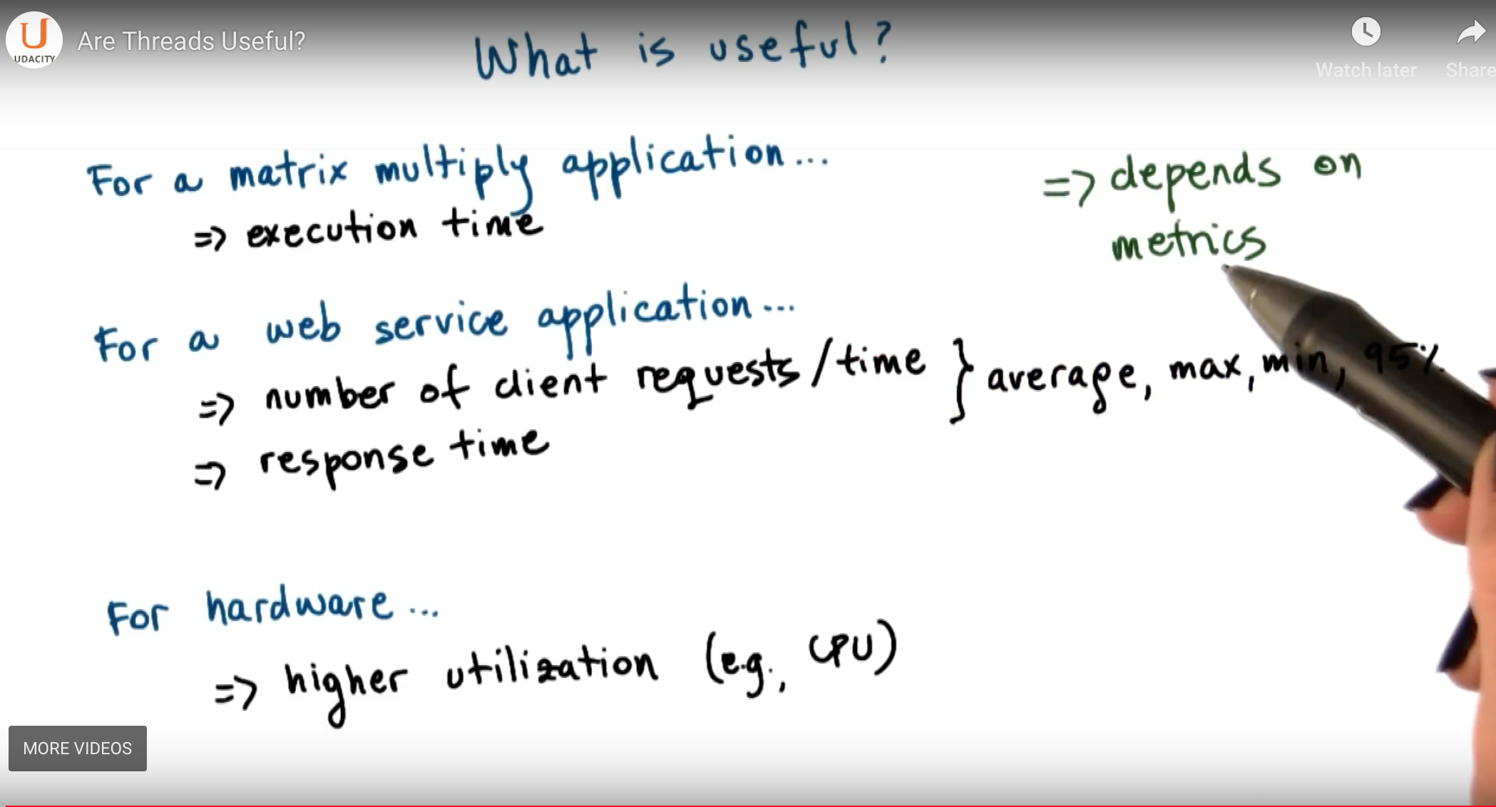
What these examples illustrate is that, to evaluate some solution, and to determine whether it’s useful or not, it is important to determine what are the properties that we really care for, what are the properties that capture the utility of that particular solution. We call such properties metrics, so basically the evaluation, and the answer to whether something is useful or not, will depend on the relevant metrics.
4 - Visual Metaphor

Let’s consider a visual metaphor in our discussion about metrics. We will do this by comparing metrics that exist in a toy shop, to metrics that exist in operating systems. For instance, from the perspective of the toy shop manager, a number of properties of how the workers operate, how the toy shop is being run, may be relevant. One example is throughput. The toy shop manager would want to make sure that this is as high as possible. Other things that may be important for the toy shop manager include how long does it take to react to a new order on average? Or what is the percentage of the workbenches that are used over a period of time? There can clearly be many more properties of the toy shop and how it’s run that are relevant to the toy shop manager. Metrics such as throughput, response time, utilization and others are also relevant from the operating systems perspective. For instance, it’s important to understand how many processes can be completed over a period of time on a particular platform.

It’s important to know how responsive the system is. So when we click the mouse, does something happen immediately or we have to wait some noticeable amount of time? Does the operating system design lead to a solution that utilizes the CPU, devices, memory well, or does it leave a lot of unused resources? So metrics exist in any type of system, and it’s important to have them well-defined when you’re trying to analyze how a system behaves and how it compares to other solutions.
5 - Performance Metrics Intro

If you have not noticed yet, performance considerations are really all about the metrics that we choose. Ideally, metrics should be represented with values that we can measure and quantify. The definition of the term metrics, according to Webster, for instance, is that it’s a measurement standard. In our analysis of systems, a metrics should be measurable. It should allow us to quantify a property of a system, so that we can evaluate the system’s behavior or at least compare it to other systems. For instance, let’s say we are concerned with the execution time of the system. That’s a metric. We can measure it. We can quantify exactly what is the execution time of a system, so it’s a quantifiable property as well. A metric is associated in some way with some system that we’re interested in. For instance, that can be the implementation of a particular problem, the software implementation of a problem. And that’s what we want to measure the execution time of. And a metric should tell us something about the behavior of the system we’re interested in. For instance, it can tell us whether it’s an improvement over other implementations of the same problem. For the later, in order to perform this kind of evaluation and comparisons, we really should explore the values of this metrics over some range of meaningful parameters. By varying the workload that this implementation needs to handle, or by varying the resources that are allocated to it, or other dimensions.
6 - Performance Metrics


So far in this lesson we mentioned several useful metrics. For instance, we talked about execution time and throughput, response time, CPU utilization. But there are many other useful metrics to consider. For instance, user may not just care when they will get an answer, but they may also care when their job will actually start being executed. We call this metric wait time. The job is interactive, so the user needs to interact with this. Obviously the sooner he starts, the sooner the user will be able to do something about it. If the job is a long running job and the sooner it starts, the user has a chance to find out maybe that something’s going wrong. So It can reconfigure the task, it can stop it and then reconfigure and launch it again. So wait time could be an important metric in some contexts. Then let’s think about throughput for instance. We know throughput helps evaluate the utility of a platform. So how many tasks will it complete over a period of time? How many processes, how many jobs will we complete at over a period of time? This can be relevant in the context of a single machine, a single server. Or in the context of an entire data center for instance. Now, if I’m the owner of the data center, throughput is not the only thing that I care for. I’m probably more concerned about some other type of metric that we can call platform efficiency. And this says some combination of how well I utilize my resources to deliver this throughput. So it’s not just a matter of having higher throughput, but also being able to utilize the resources that are available in my data center more efficiently. The reason for this is that as a data center operator, I make money when I complete jobs. So the higher the throughput, the greater the income for me. However, I also spend money to run the machines, to buy more servers. So it’s important to have a good ratio. So platform efficiency would for instance, capture that. If it’s really just the dollars that I’m concerned about, then a metric like performance per dollars would capture that. So if I’m considering buying the next greatest hardware platform. Then I can think about whether the cost that I will pay extra for that new piece of hardware, will basically be compensated with some impact on the performance that I see. Or maybe I’m concerned about the amount of power, the watts, that can be delivered to a particular platform. Or the energy that will be consumed during the execution. So then defining some metrics that capture performance per watt, or performance per joule will be useful ones. You may have heard of the term SLA. It stands for Service Level Agreement. Enterprise applications will give typically SLAs to their customers. One example, for instance will be that you will get a response within three seconds. Or, it may be even more subtle than that. For instance, a service like Expedia perhaps, has an SLA with it’s customers. And it’s customers would be like Delta Airlines and American Airlines, that it will provide most accurate quote for 95% of the flights that are being returned to customers. So then for that enterprise application, one important thing would be whether there any SLAs that are violated. Whether there are any customer requests that took longer than three seconds, or that did not provide quotes for airfare that were all 100% accurate. A metric-like percentage of SLA violations would capture that information. For some applications, there is some natural opportunity for a slack in the application. For instance, if you think about a regular video application, humans can’t perceive more than 30 frames per second. So being so focused on the frames per second, and trying to maximize that frames per second rate, that’s not the goal. However, making sure that there’s at least 30 frames per second. So that users don’t start seeing some random commercials during the video that they’re watching on YouTube, that’s something that’s important. So it’s not so much about this raw request rate or wait time, but rather it’s a metric that really is concerned whether the client perceives the service as performing well or not. You may be concerned with the performance metric of an individual application. Or you may need to try to come up with some kind of aggregate performance metric that tries to average the execution time for all tasks, or average the wait time for all tasks. Or maybe even this would be a weighted average based on the priorities of the tasks. Also in addition to just being constrained with CPu utilization, there are a number of other resources that we may be concerned about. Memory, file systems, the storage subsystem. So some metrics that are concerned with the average resource usage are also useful
7 - Performance Metrics Summary
In summary a metric is some measurable quantity that we can use to reason about the behavior of the system. Ideally we will obtain these metrics. We will gather these measurements running experiments using real software deployment on the real machines using real workloads. However sometimes that’s really not an option. We cannot wait to actually deploy the software before we start measuring something about it or analyzing its behavior. In those cases we have to resort to experimentation with some representative configurations that in some way mimic as much as possible the aspects of the real system. The key here is that such a toy experiment must be representative of this real environments so we must use workloads that have similar access patterns, similar types of machines. So as closely mimics the behavior of the real system as possible. And possibly we will have to supplement those toys experiments with simulation. So that we can perhaps create an environment that somehow mimics up a larger system that was possible with a small experiment. Any of these methods represent viable settings where one can evaluate a system and gather some performance metrics about t. We refer to these experimental settings as a testbed. So the testbed that tells us where were the experiments carried out and what were the relevant metrics that were measured?
8 - Really… Are Threads Useful?

So if we go back now to our question, are threads useful? We realize that the answer is not so simple. We cannot simply say, yes, threads are useful. We know that the answer of the question will depend on the metrics that we’re interested in. Also, it will depend on the workload. We saw in the toy shop example where we compared the boss worker and the pipeline model that the answer as to which model is better dependent on the number of toys that need to be processed to the number of orders. So in the toy shop example, depending on the workload, the toy orders, and metrics we were concerned in, it lead us to conclusion that a different implementation of the toy shop, a different way to organize its workers was a better one. If you look at other domains, for instance, if we think about graphs and graph processing. Depending on the kind of graph, how well connected it is, it may be suitable to choose different type of shortest path algorithm. Some shortest path algorithms are known to work well on densely connected graphs whereas others work better for sparsely connected graphs. So again, the workload is something that we’re interested in. When comparing file systems, maybe what’s important to consider is the, the patterns. The file, some file systems may be better for predominantly read accesses whereas others are better for more of a mixed workload, where files are both read and updated. The point of looking at all of these is that across the board, both for the first question as well as in these other cases, the answer of whether something is better than an alternative implementation or an algorithm, it’s pretty much always it depends. Depending on the file pattern, depending on the graph, depending on the number of toy orders. So similarly, the answer to, are threads useful isn’t really going to be a straightforward yes and no one. It’s really going to depend on the context in which we’re trying to answer this question. And while we are at this, it depends, answer, you should know that it’s pretty much always the correct answer to a question in systems. However, it’s never going to be an accepted one. I will not take it as accepted answer in this course either. For the remainder of this lecture, we will to answer a specifically, whether threads are useful. And when are threads more or less useful when comparing a multithreaded-based implementation of a problem to some alternatives. I will also provide you with some guidance on how to define some useful metrics, and how to structure experimental evaluations, so that you can correctly measure such metrics.
Multi Process vs Multi Threads


To understand Winter threats useful, let’s start to think about what are the different ways to provide concurrency and what are the trade offs among those implementation. So far we’ve talked about multi threaded applications. But an application can be implemented by having multiple concurrently running processes. We mentioned this in the earlier lecture on Threads and Concurrency. So let’s start by comparing these two models. To make the discussion concrete we will do this analysis in the context of a web server. And for a web server it’s important to be able to concurrently process client requests. So that is the concurrency that we care for there. Before we continue let’s talk for a second about what are the steps involved in the operation of a simple web server. At the very first, the client or the browser needs to send a request that the web server will accept. So let’s say this is a request to www.contact.edu and the web server at Georgia Tech needs to accept that request. After the request is accepted, there are a number of processing steps that the web server needs to perform before finally responding with the file. Now, we will talk about a simple web server. So if we take a look at what these steps are, so we accept the connection, we read the request that there is an HTTP request that’s received and we need to parse that request. We need to then find the file in the local file system, that’s at the server side. Once we have extracted the file, we need to compute the header, send out the header and then also send out the file or potentially send out an error message along with the header that the file is not found. So for the rest of this lesson we’ll really focus on this simple web server processing. One of the things that’s worth pointing out is that there’s some differences among these steps. Some of them are more computational intensive, so it’s mostly, the work is done by the CPU. For instance, parsing the request or computing the header. This is mostly done by the CPU. Other steps may require some interaction with the network, like accepting connection, reading request, or sending the data. Or the disk, for instance, when finding the file and then reading the file from the disk. These steps may potentially block, but whether or not they block will really depend on what is the state of the system at a particular point of time. So for instance, the connection may already be pending or the data for the file may already be cached in memory because of the previous request that serviced that file. So in those cases, these will not result in an actual call to the device, so an actual implication of the disk or the network and will be serviced much more quickly. Once the file or potentially the error message are sent out to the client, then the processing is complete.
10 - Multi Process Web Server

This, then, clearly represents a single threaded process. One easy way to achieve concurrency is to have multiple instances of the same process. And that way we have a multi-process implementation. This illustration is adapted from Vivek Pai’s paper, Flash, An Efficient and Portable Web Server, and it appears as figure two in the paper. The benefits of this approach is that it is simple. Once we have correctly developed the sequence of steps for one process, we just spawn multiple processes. There are some downsides, however, with running multiple processes in a platform. We’ll have to allocate memory for every one of them and this will ultimately put high load on the memory subsystem and it will hurt performance. Given that these are processes, we already talked about the cost of context switch among processes. Also it can be rather expensive to maintain shared state across processes because the communication mechanisms and the synchronization mechanisms that are available across processes, those are little bit higher overhead. And in some cases it may even be a little bit tricky to do certain things like, for instance, forcing multiple processes to be able to respond to a single address and to share an actual socket port.
11 - Multi Threaded Web Server


An alternative to the multi-process model is to develop the web server as a multi-threaded application. So here we have multiple execution context, multiple threads within the same address space and every single one of them is processing a request. Again, this illustration is taken from Pai’s Flash paper, and this is figure three there. In this figure, every single one of the threads executes all the steps, starting from the accept connection call all the way down to actually sending the file. Another possibility is to have the web server implemented as a boss-workers model where a single boss thread performs the accept connection operation. And every single one of the workers performs the remaining operations from the reading of the HTTP request that comes in on that connection until actually sending the file. The benefits of this approach is that the threads share the address space, so they will share everything that’s within it. They don’t have to perform system calls in order to coordinate with other threads, like what’s the case in the multi-threaded execution. Also context switching between these threads is cheap. It can be done at the user level, threading library level. Because a lot of the per thread state is shared among them, then we don’t have to allocate memory for everything that’s required for each of these execution contexts. They share the address space, so the memory requirements are also lower for the multi-threaded application. The downside of the approach is that it is not simple and straightforward to implement the multi-threaded program. You have to explicitly deal with synchronization when threads are accessing and updating the shared state. And we also rely for the underlying operating system to have support for threads. This is not so much of an issue today. Operating systems are regularly multi-threaded. But it was at the time of the writing of the Flash paper, so we will make sure that we address this argument as well in our explanations.
12 - Event-Driven Model


Now let’s talk about an alternative model for structuring server applications that perform concurrent processing. The model we’ll talk about is called event-driven model. An event-driven application can be characterized as follows. The application is implemented in a single address space, there is basically only a single process. And a single thread of control. Here is the illustration of this model and this is taken from the read pies flash paper as well. The main part of the process is the event dispatcher that continuously in a loop looks for incoming events and then based on those events invokes one or more of the registered handlers. Here events correspond to some of the following things. We see that the request from the client browsers, that message that’s received from the network, that’s an event. Completion of the send, so once the server responds to the client request, the fact that the send completed, that’s another event, as far as the system is concerned. Completion of a disk read operation. That’s another event that the system will need to know how to handle. The dispatcher has the ability to accept any of these types of notifications, and then based on the notification type to invoke the appropriate handler. So in that sense, it operates very much like a state machine. Since we’re talking about a single credit process, invoking a handler simply means that we will jump to the appropriate location in the processes address space where the handler is implemented. At that point the handler execution can start. For instance, if the process is notified that there is a pending connection request on the network port that it uses, the dispatcher will pass that event to the accept connection handler. If the event is a receipt of a data of message on an already established connection, then the event dispatcher will pass that to the read request handler. Once the filename is extracted from the request and it’s confirmed that the file is present, the process will send out chunks of the file. And then once there is a confirmation that that chunk of the file portion of the file has been successfully sent and it will continue iterating over the handler that’s dealing with the send operation. If the file is not there, then some sort of error message will be sent to the client. So whenever an event occurs the handlers are the sequence of code that executes in response to these events. The key feature of the handlers is that they run to completion. If a handler needs to perform a blocking operation, it will initiate the blocking operation and then it will immediately pass control back to the event dispatcher, so it will no longer be in the handler. At that point, the dispatcher is free to service other events or call other handlers.
13 - Concurrency in the Event Driven Model


You’re probably asking yourselves, if the event-driven model has just one thread, then how did it achieve concurrency? In the multi-process and the multi-threaded models, we had each execution context, whether it’s a process or a thread, handle only one request at a time. To achieve concurrency, we would simply add multiple execution context, so multiple processes or multiple threads. And then, if necessar,y if we have fewer CPUs than contexts, then we would have to context-switch among them. The way the event-driven model achieves concurrency is by interleaving the processing of multiple requests, within a same execution context. Here in the event-driven model, we have a single thread, and the single thread switches its execution among the processing that’s required for different requests. Let’s say we have a client request coming into the system, so it’s a request for client C1. And we receive a request for a connection that gets dispatched, the accept operation gets processed. Then, we receive the actual request. So it’s an HTTP message that gets processed, the message gets parsed, we extract the files. So now we actually need to read the file and we initiate I/O from the reading file handler. So at that point, the request for client one has been processed through several of these steps and it’s waiting on the disk I/O to complete. Let’s say, in the meantime, two more requests have come in. So client two and client three have sent a request for a connection. Let’s say the client two request was picked up first, the connection was accepted, and now for the processing of client two, we need to wait for the actual HTTP message to be received. So the processing of client two is waiting on an event from the network that will have the HTTP message that needs to be received. And let’s say client three, its request has been accepted and it’s currently being handled, so the client three request is in the accept connection handler. Some amount of time later, the processing of all of these three requests has moved a little bit further along. So the request for C3, the accept connection was completed, and now that request is waiting on an event with the HTTP message. The request for client two, that one, perhaps, we’re waiting on the disk I/O, in order to read the file that needs to be sent out. And maybe the request for client C1, already started sending the file in chunks at a time, so blocks of some number of bytes at a time. So, it’s waiting in one of those iterations. So, although we have only one execution context, only one thread, if we take a look, we have concurrent execution of multiple client requests. It just happens to be interleaved, given that there’s one execution context. However, they’re multiple, at the same time, multiple client requests being handled.
14 - Event-Driven Model: Why

The immediate question is why does this work. What is the benefit of having a single thread that’s just going to be switching among the processing of different requests compared to simply assigning different requests to different execution contexts, to different threads or even to different processings. Recall our introductory lecture about threads, in which we said that on a single CPU threads can be useful because they help hide latency. The main takeaway from that discussion was that, if a thread is going to wait more than twice the amount of time it takes to perform a contact switch, then it makes sense to go ahead and context switch it to another thread that will do some useful work. And in that way we hide this waiting latency. If there really isn’t any idle time. So if the processing of a request doesn’t resolve in some type of blocking idle operation on which it has to wait, then there are no idle periods. It doesn’t make sense to context switch. The context switching time will be just cycles that are spent on copying and restoring a thread or a process information, and those cycles could have been much better spent actually performing request processing. So in the event driven model, a request will be processed in the context of a single thread, as long as it doesn’t have to wait. Whenever a wait needs to happen, then the execution thread will switch to servicing another request. If we have multiple CPUs, the event driven model still makes sense, especially when we need to handle more concurrent requests than the number of CPUs. For instance, each CPU could host a single event-driven process, and then handle multiple concurrent requests within that one context. And this could be done with less overhead than if each of the CPUs had to context-switch among multiple processes or multiple threads where each of those is handling a separate request. There is one gotcha, though, here. It is important to have mechanisms that will steer, that will direct the right set of events to the appropriate CPU, at the appropriate instance of the event-driven process. And there are mechanisms to do this, and there’s current support, a networking hardware to do these sorts of things, but I’m not going to go into this in any further detail. So just know that overall in the model, this is how the event-driven model would be applied a multi-CPU environment.
15 - Event-Driven Model: How


Now let’s see how can this be implemented. So at the lowest level, we need to be receiving some events, some messages from the network or from the disk. So information about completed requests to read a portion of the file, write the file, etc. The operating systems use these two abstractions to typically represent networks or disks. So sockets are typically used to represent interface to the network. And then files are what’s really stored on disks. So these are the main abstractions when it comes to storage. Now although they are called differently, sockets and files, it is quite fortunate that internally, the actual data structure that’s used to represent these two different obstructions, is actually identical. It’s called the file descriptor. So then an event in the context of this web server is an input on any of the files descriptors that are associated with it. So in any of the sockets. Or any of the files that are being accessed by the connections that these sockets carry. To determine which file descriptor has input, so to determine that there is an event that has arrived in this system. The flash talks about using the select call. The select call takes a range of file descriptors and then returns the very first one that has some kind of input on it. And that is regardless is whether that file descriptor is a socket or a file ultimately. Another alternative to this is to use a poll API. So this is another system call that’s provided by current operating systems. The problem with both of these, is that they really have to scan through potentially really large list of file descriptors, until they find one. And, it is very likely that along that long list of file descriptors, there going to be only very few that have inputs. So, a lot of that search time will be wasted. An alternative to these is a more recent type of API that’s supported by, for instance, the Linux kernel and that’s e poll so this eliminates some of the problems that select and poll have. And a lot of the high performance servers that require high data rates and low latency use this kind of mechanism today. The benefits of the event driven model really come from its design. It’s a single address space, single flow of control. As a result, the overheads are lower. There’s no need for context switching. Overall, it’s a much more compact process so it has smaller memory requirements. And the programming is simpler. We don’t need to worry about use of synchronization primitives, about shared access to variables, etc. Now, in the context of this single thread, we are switching among multiple connections, so we are jumping all over the code base of this process and executing different handlers, accessing different states. That will have some effect on basically loss of localities and cache pollution effects. However, that will be significantly lower than would have been happening if we were doing a full blown context switching. So the overheads and some of the elimination of the synchronization, these are some of the things that really make this an attractive approach.
16 - Helper Threads and Processes


The event-driven model doesn’t come without any challenges. Recall that when we talked about the many to one multithreading model, we said that a single blocking I/O call that’s coming from one of the user level threads can block the entire process, although there may be other user level threads that are ready to execute. A similar problem can occur here as well. If one of the handlers issues a blocking I/O call to read data from the network or from disk, the entire event-driven process can be blocked. One way to circumvent this problem, is to use asynchronous I/O operations. Asynchronous calls have the property that when the system call is made, the kernel captures enough information about the caller and where and how the data should be returned once it becomes available. Async calls also provide the caller with an opportunity to precede executing something, and then come back at a later time to check if the results of the asynchronous operation are already available. For instance, the process or the thread can come back later to check if a file has already been read and the data is available in the buffer in memory. One thing that makes asynchronous calls possible is that the OS kernel is multithreaded. So while the caller thread continues execution, another kernel thread does all the necessary work and all the waiting that’s needed to perform the I/O operation, to get the I/O data, and then, to also make sure that the results become available to the appropriate user level context. Also, asynchronous operations can benefit by the actual I/O devices. For instance, the caller thread can simply pass some request data structure to the device itself, and then the device performs the operation, and the thread at a later time can come and check to see whether device has completed the operation. We will return to a synchronous I/O operations in a later lecture. What you need to know for now is that when we’re using asynchronous I/O operations, our process will not be blocked in the kernel when performing I/O. In the event-driven model, if the handler initiates an asynchronous I/O operation for network or for disk, the operating system can simply use the mechanism like select or poll or epoll like we’ve mentioned before to catch such events. Since summary asynchronous I/O operations fit very nicely with the event-driven model. The problem with asynchronous I/O calls is that they weren’t ubiquitously available in the past. And even today, they may not be available for all types of devices. In a general case, maybe the processing that needs to be performed by our server isn’t to read data from a file, where there are asynchronous system calls. But instead maybe to call processing some accelerator, some device that only the server has access to. To deal with this problem, paper proposed the use of helpers. But a handler needs to issue an I/O operation that can block, it passes it to the helper, and returns to the event dispatcher. The helper will be the one that will handle the blocking I/O operation, and interact with the dispatcher as necessary. The communication with the helper can be via socket based interface, or via another type of messaging interface that’s available in operating systems called pipes. And both of these present a file descriptor-like interface. So the same kind of select or poll mechanism that we mentioned can be used for the event dispatcher to keep track of various events that are occurring in the system. This interface can be used to track whether the helpers are providing any kind of events to the event dispatcher. In doing this, the synchronous I/O call is handled by the helper. The helper will be the one that will block, and the main event dispatcher in the main process will continue uninterrupted. So this way although we don’t have asynchronous I/O calls, through the use of helpers, we achieve the same kind of behavior as if we had asynchronous calls. At the time of the writing of the paper, another limitation was that not all kernels were multi-threaded. So basically, not all kernels supported the one to one model that we talked about. In order to deal with this limitation, the decision in the paper was to make these helper entities processes. Therefore, they call this model AMPED, Asymmetric Multi-Process Event-Driven model. It’s an event-driven model. It has multiple processes. And these processes are asymmetric. The helper ones only deal with blocking I/O operation. And then, the main one performs everything else. In principle, the same kind of idea could have applied to the multi-threaded scenario where the helpers are threads, not processes, so asymmetric multi-threaded event-driven model. And in fact, there is a follow-on on the Flash work that actually does this exact thing, the AMTED model. The key benefits of the symmetric model that we described is that it resolved some of the limitations of the pure event-driven model in terms of what is required from the operating system, the dependence on asynchronous I/O calls and threading support. In addition, this motto lets us achieve concurrency with a smaller memory footprint than either the multi-process or the multi-threading model. In the multi-process or multi-threading model, a worker has to perform everything for a full request. So its memory requirements will be much more significant than the memory requirements of a helper entity. In addition, with the AMPED model, we will have a helper entity only for the number of concurrent blocking I/O operations. Whereas, in the multi-threaded or multi-process models, we will have as many current entities, as many processes, or as many threads as there are concurrent requests regardless of whether they block or not. The downside is that audit works well with the server pipe applications. It is not necessarily as generally applicable to arbitrary applications. In addition, there are also some complexities with the routing of events in multi CPU systems.
17 - Models and Memory Quiz
Here is a quick quiz analyzing the memory requirements of the three concurrency models we talked about so far. The question is, of the three models mentioned so far, which model likely requires least amount of memory? The choices are the Boss-Worker Model, the Pipeline Model and the Even-Driven Model. Also answer why you think that this model requires the least amount of memory to see if your reasoning matches ours.
18 - Models and Memory Quiz Solution

The correct answer is that likely the event-driven model will consume least resources. Recall that in the other models, we had a separate thread for each of the requests or for each of the pipeline stages. In the event-driven model, we have handlers which are just procedures in that address space, and the helper threads only occur for blocking I operations. For the event-driven model, extra memory is required only for the helper threads that are associated with concurrent blocking I/O calls. In the boss-worker model, extra memory will be required for threads for all concurrent requests, and similarly, even in the pipeline model, concurrent requests will demand multiple threads to be available in a stage of the pipeline if the level of concurrency is beyond the number of pipeline stages. As a result, the event-driven model will likely have the smallest memory footprint.
19 - Flash Web Server


With all this background on the event-driven model, we will now talk about the Flash paper. Flash is an event-driven webserver that follows the AMPED model, so basically it has asymmetric helper processes to deal with the blocking guy operations. In the discussion so far, we really described the architecture of Flash. So it uses helper processes for blocking I/O operations. And then everything else is implemented as an event dispatcher with handlers performing different portions of the web servicing tasks. Given that we are talking about a web server, and this is the old fashioned Web 1.0 technology where basically the web server just returns static files. The blocking I operations that are happening an the system are really just disk reads, so the server just reads files that the client requests. The communication from the helpers to the event dispatcher is performed via pipes. The helper reads the file in memory via the mmap call, and then the dispatcher checks the in-operation mincore, if the pages of the file are in memory. And it then uses this information to decide if it should just call one of the local handlers, or if it should pass the request to the helper. As long as the file is in memory, reading it won’t result in a blocking I/O operation, and so passing it to the local handlers is perfectly okay. Although this is an extra check that has to be performed before we read any file, it actually results in big savings because it prevents the full process from being blocked if it turns out that a blocking I/O operation is necessary. Now we will outline some additional detail regarding some of the optimization that Flash applies. And this will help us later understand some of the performance comparisons. The important thing is that these optimizations are really relevant to any web server. First of all, Flash performs application-level caching at multiple levels. And it does this on both data and computation. What we mean by this is, it’s common to cache files. This is what we call data caching. However, in some cases it makes sense to cache computation. So in the case of the web server, the requests are requests for some files. These files need to be repeatedly looked up. So you need to find the file, traverse the directory, look up some of the directory data structures. That processing will compute some results. So some location, some pathname for the file. And we will just cache that. We don’t have to recompute that and look up the same information next time a request for that same file comes in. Similarly in the context of web processing, the HTTP header that files have that are returned to the browser, it’s really going to depend on the file itself. So a lot of the fields in there are file dependent given that the file doesn’t change. The header doesn’t have to change so this is another type of application level caching that we can perform and Flash does this. Also Flash does some optimizations that take advantage of the networking hardware and the network interface card. For instance all of the data structures are aligned so that it’s easy to perform DMA operations without copying data. Similarly, they use DMA operations that have scatter-gather support, and that really means that the header and the actual data don’t have to be aligned one next to another in memory. They can be sent from different memory locations, so there’s a copy that’s avoided. All of these are very useful techniques, and are now fairly common optimizations. However, at the time the paper was written, they were pretty novel, and in fact, some of the systems they compare against did not have some of these things included.
20 - Apache Web Server

Before we continue I would like to briefly describe the Apache Web Server. It’s a popular open source web server, and it’s one of the technologies that in the flash paper the author’s compare against. My intent is not to give a detailed lecture on Apache. That’s beyond the scope of the course, but instead I wanted to give you enough about the architecture of Apache, and how it compares to the models that we discussed in the class. And also the other way around, to understand how these discussions in class, are reflected in real world designs. From a very high level, the software architecture of Apache looks like this. The core component provides the basic server-like capability, so this is accepting connections and managing concurrency. The various modules correspond to different types of functionality that is executed on each request. The specific Apache deployment can be configured to include different types of modules. For instance, you can have certain security features, some management of dynamic content, or even some of the modules are really responsible for more basic HTP request processing. The flow of control is sort of similar to the event driven model that we saw, in the sense that each request passes through all of the modules. Like in the event driven module each request ultimately passed through all the handlers. However, Apache’s a combination of a multiprocess and a multithreaded model. In Apache, a single process, a single instance, is internally a multithreaded, boss/worker process that has dynamic management of the number of threads. There’s some configurable thresholds that can be used to dynamically track when to increase or decrease the number of threads in the pool. The total number of processes, so the MP part of the model, can also be dynamically adjusted, and for these, it’s information such as number of outstanding connections, number of pending requests, CPU usage, a number of factors can drive how the number of the threads per process and the total number of processes are adjusted.
21 - Experimental Methodology


It is now time to discuss the experimental approach in the Flash paper. In the paper, the experiments are designed so that they can make stronger arguments about the contributions that the authors claim about Flash. And this is something that you should always consider when designing experiments. That they should help you with the arguments that you’re trying to make. To do this, to achieve a good experimental design, you need to answer a number of questions. For instance, you should ask yourself, what is it that you’re actually comparing? Are you comparing two software implementations? The hardware the same. Are you comparing two hardware platforms? Make sure then the software is the same. You need to outline the workloads that will be used for evaluation. What are the inputs in the system? Are you going to be able to run data that resembles what’s seen in the real world or are you going to generate some synthetic traces? These are all important questions you need to resolve. Not to forget the metrics, we talked about them earlier in this lesson is that execution time or throughput or response time. What is it that you care for and who are you designing this system for? Is it the manager? Is it resource usage in the system? Or is it ultimately the customer’s? So let’s see now how these questions were treated in the Flash paper. Let’s see what were the systems that they were comparing, what were the comparison points? First they include a comparison with a multiprocess version of the same kind of Flash processing. So a web server with the exact same optimizations that were applied in Flash however, in a multiprocess, single-threaded configuration. Then again, using the same optimizations as Flash, they put together a multithreaded web server that follows the boss-worker model. Then they compare Flash with a Single Process Event-Driven model, so this is like the basic event-driven model that we discussed first. And then they also use as a comparison, two existing web server implementations. One was a more research implementation that followed the SPED model, however it used two processes and this was to deal with the blocking I/O situation. And then another one was Apache and this is the open-source Apache web server. And this was at the time when this was then an older version obviously than what’s available today and at the time Apache was a multiprocess configuration. Except for Apache, every single one of these implementations integrated some of the optimizations that Flash already introduced. And then, every single one of these implementations is compared against Flash. So this basically means, is that they’re comparing the different models, multiprocess, multithreaded SPED against the AMPED, the asymmetric multiprocess event-driven model. Given that all of these really implement, otherwise the exact same code with the same optimizations. Next let’s see what are the workloads they chose to use for the evaluations. To define useful inputs, they wanted workloads that represent a realistic sequence of requests. Because that’s what will capture our distribution of web page accesses. But they wanted to be able to reproduce, to repeat the experiment with the same pattern of accesses. Therefore, they used a trace-based approach where they gathered traces from real web servers. And then they replayed those traces so as to be able to repeat the experiment with the different implementations. So that every single one of the implementations can be evaluated against the same trace. What they ended up with were two real world traces, they were both gathered at Rice University where the authors are from, actually were from. Some of them are no longer there. The first one was the CS web trace, and the second one was the so-called Owlnet trace. The CS trace represents the Rice University Web Server for the Computer Science Department. And it includes a large number of files and it doesn’t really set in memory. The Owlnet trace, that one was from a web server that hosted the number of student webpages. And it was much smaller, so would typically fit in the memory of common server. In addition to these two traces, they also use the synthetic workload generator. And with the synthetic workload generator, as opposed to replaying these traces of real world page access distributions. They would perform some best or worst type of analysis, or run some what if questions. Like what if the distribution of the web pages accesses had a certain pattern, would something change about their observations? And finally, let’s look at what are the relevant metrics that the authors picked in order to perform their comparisons. First, when we talk about web servers, a common metric is clearly bandwidth. So what is the total amount of useful bytes or the bytes transferred from files, over the time that it took to make that transfer? And the unit is clearly bytes per second, megabytes per second and similar. Second, because they were particularly concerned with Flash’s ability to deal with concurrent processing. They wanted to see the impact on connection rate as a metric. And that was defined as the total number of client connections that are serviced over a period of time. Both of these metrics were evaluated as a function of the file size, so the understanding they were trying to gain was. How does the workload property of requests that are made for different file sizes impact either one of these metrics? The intuition is that with a larger file size, the connection cost can be ammortize. And that you can at the same time push out more bytes, so you can basically obtain higher bandwidth. However, at the same time the larger the file, the more work that the server will have to do for each connection. Because it will have to read and send out more bytes from that larger file. So that will potentially negatively impact the connection rate. So this is why they chose that file size was a useful parameter to vary. And then understand it’s impact on these metrics for the different implementations.
22 - Experimental Results


Let’s now look at the experimental results. We will start with the best case numbers. To gather the best case numbers, they used a synthetic load in which they varied the number of requests that are issued against the web server, and every single one of the requests is for the exact same file. Like for instance, every single one of the requests is trying to get index.html. This is the best case because really in reality clients will likely be asking for different files, and in this pathological best case it’s likely basically the file will be in cash so every one of these requests will be serviced as fast as possible. There definitely won’t be any need for any kind of disk IO. So for the best case experiments, they measure bandwidth and they do that, they vary the file size of zero to 200 kilobytes and they measure bandwidth as the n, the number of requests, times the file size over the time that it takes to process the n number of requests for this file. By varying the file size, they varied the work that both the web server performs on each request but also the amount of bytes that are generated on a request. You sort of assume that as we increase the file size that the bandwidth will start increasing. So let’s look at the results now. The results show the curves for every one of the cases that they compare. The flash results are the green bar, SPED is the single process event driven model, MT, multi-threaded, MP, multi-process, Apache, this bottom curve, corresponds to the Apache implementation And Zeus, that corresponds to the darker blue. This is the SPED module that has two instances of SPED so the dual process event driven model. We can make the following observations. First, for all of the curves, initially when the file size is small, bandwidth is slow, and as the file size increases, the bandwidth increases. We see that all of the implementations have very similar results. SPED is really the best. That’s the single process event driven, and that’s expected because it doesn’t have any threads or processes among which it needs to context switch. Flash is similar but it performs that extra check for the memory presence. In this case, because this is the single file tree. So every single one of the requests is for the single file, there’s no need for blocking I/O. So none of the helper processes will be invoked, but nonetheless, this check is performed. So that’s why we see a little bit lower performance for flash. Zeus has an anomaly. Its performance drops here a little bit, and that has to do with some misalignment for some of the DMA operations. So not all of the optimizations are bug-proof in the Zeus implementation. For the multi-thread and multi-process models, the performance is slower because of the context switching and extra synchronization. And the performance of Apache is the worst, because it doesn’t have any optimizations that the others implement. Now, since real clients don’t behave like the synthetic workload, we need to look at what happens with some of the realistic traces, the Owlnet and the CS trace. Let’s take a look at the Owlnet trace first. First we see that for the Owlnet trace, the performance is very similar to the best case with SPED and Flash being the best and then Multi-thread and Multi-process and Apache dropping down. Note that we’re not including the Zeus performance. The reason for this trend is because the Owlnet trace is the small trace, so most of it will fit in the cache and we’ll have a similar behavior like what we had in the best case, where all the requests are serviced from the cache. Sometimes, however, blocking I/O is required. It mostly fits in the cache. Given this, given the blocking I/O possibility, SPED will occasionally block. Where as in Flash their helper processes will help resolve the problem. And that’s why we see here that the performance of Flash is slightly higher than the performance of the SPED. Now if we take a look at what’s happening with the CS trace, this, remember, is a larger trace. So it will mostly require I/O. It’s not going to fed in the cache, in memory in the system. Since the system does not support asynchronous I/O operations, the performance of SPED will drop significantly. So relative to where it was, close to Flash, now it’s significantly below Flash and, in fact, it’s below the multi-process and the multi-threaded implementations. Considering the multi-thread and the multi-process, we see that the multi-threaded is better than the multi-process, and the main reason for that is that the multi-threaded implementation has a smaller memory footprint. The smaller memory footprint means that there will be more memory available to cache files, in turn that will lead to less I/O, so this is a better implementation. In addition, the synchronization and coordination and contact switching between threads in a multi-thread implementation is cheaper, it happens faster than long processes in a multi-process implementation. In all cases, Flash performs best. Again, it has the smaller memory footprint compared to multi-threaded and the multi-process, and that results in more memory available for caching files or caching headers. As a result of that, fewer requests will lead to a blocking I Operation which further speeds things up. And finally, given that everything happens in the same address space, there isn’t a need for explicit synchronization like with the multi-threaded or multi-process model. And this is what makes Flash perform best, in this case. In both of those cases, Apache performed worse, so let’s try to understand if there’s really an impact of the optimizations performed in Flash. And here the results represent the different optimizations. The performance that’s scattered with Flash without any optimizations that’s the bottom line. Then Flash with the path only optimizations, so the path only, that’s the directory lookup caching, so that’s like the computation caching part. Then the red line here, the path and maps, so this includes caching of the directory lookup plus caching of the file. And then the final bar, so the final line, the black line, that includes all of the optimization. So this is the directory lookup, the file caching as well as the header computations of the file. And we see that as we add some of the optimizations, this impacts the connection rates of the performance that can be achieved by the web server significantly improves. We’re able to sustain a higher connection rate as we add these optimizations. This tells us two things. First, that these optimizations are indeed very important. And second, they tell us that the performance of Apache would have been also impacted, if it had integrated some of these same optimizations as the other implementations.
23 - Summary of Performance Results

To summarize, the performance results for Flash show the following. When the data is in cache, the basic SPED model performs much better than the AMPED Flash, because it doesn’t require the test for memory presence, which was necessary in the AMPED Flash. Both SPED and the AMPED Flash are better than the multi-threaded or multi-process models, because they don’t incur any of the synchronization or context switching overheads that are necessary with these models. When the workload is disk-bound, however, AMPED performs much better than the single-process event-driven model, because the single process model blocks, since there’s no support for asynchronous I/O. AMPED Flash performs better than both the multi-threaded and the multi-process model, because it has much more memory efficient implementation, and it doesn’t require the same level of context switching as in these models. Again, only the number of concurrent I/O bound requests result in concurrent processes or concurrent threads in this model. The model is not necessarily suitable for every single type of server process. There are certain challenges with event-driven architecture. We said, some of these can come from the fact that we need to take advantage of multiple cores and we need to be able to route events to the appropriate core. In other cases, perhaps the processing itself, is not as suitable for this type of architecture. But if you look at some of the high performance server implementations that are in use today, you will see that a lot of them do in fact use a event-driven model, combined with a synchronous I/O support.
24 - Performance Observation Quiz
Let’s take one last look at the experimental results from the flash paper as a quiz this time. Here’s another graph from the Flash paper and focus on the green and the red bars that correspond to the Single-Process Event-Driven model and the Flash-AMPED model. You see that about 100 megabytes, the performance of Flash becomes better than the performance of the SPED model. Explain why, and you should check all that apply from the answers below. Flash can handle I/O operations without blocking. At that particular time, SPED starts receiving more requests. The workload becomes I/O bound. Or, Flash can cache more files.
25 - Performance Observation Quiz Solution

The first answer is correct, yes. Flash has the helper processes, so it can handle I operations without blocking. The second answer really makes no sense. Both processes continue receiving the same number of requests in these experiments. The third answer is correct as well. At 100 megabytes, the workload, it’s size increases. It cannot fit in the cache as much as before, and so it becomes more I/O bound. There are more I/O requests that are needed beyond this point. For a SPED, at this point, once the workload starts becoming more O/I bound the problem is that a single blocking i operation will block the entire process. None of the other requests can make progress, and that’s why its performance significantly drops at that point. And finally, the last answer, that flash can handle more files. That’s really not correct. SPED and Flash have comparable memory footprints. And so, it is not that one can handle more files than the other in the memory cache. If anything, Flash has the helper processing so if those are created, they are going to interfere with the other available memory, and will impact the number of available cache in the negative sense. So if anything, it will have less available memory for caching files than SPED, so this is not an answer that explains why the Flash performance is better than the SPED performance.
26 - Advice on Designing Experiments


Before we conclude this lesson I’d like to spend a little more time to talk about designing experiments. It sounds like it’s easy, we just need to run bunch of test cases, gather the metrics, and show the results. Not so fast actually, you running tests, gathering metrics and plotting the results. It’s not as straightforward as it might seem. There is actually a lot of thought and planning that should go into designing relevant experiments. By relevant experiment, I’m referring to an experiment that will lead to certain statements about a solution. That are credible, that others will believe in, and that are also relevant that they will care for. For example, the paper we discussed is full of relevant experiments. There the authors provided the detailed descriptions of each of the experiments. So that we could understand them and then we could believe that those results are seen. And then we were also able to make well founded statements about flash and the ambit model versus all of the other implementations. Let’s continue talking about the web server as an example for which we’ll try to justify what makes some experiments relevant. Well, the clients using the Web Server. They care for the response time. How quickly do they get a web page back? The operators, for instance, running that Web Server, that website. We care about throughput, how many total client requests can see that webpage over a period of time? So this illustrates that you will likely need to justify your solution, using some criteria that’s relevent to the stakeholders. For instance, if you can show that your solution improves both response time and throughput, everybody is positively impacted, so that’s great. If you can show that your solution only improves response time but doesn’t really affect throughput, well okay. I’ll buy that too. It serves me some benefit. If I see a solution that improves response time and actually degrades throughput, that still could be useful. Perhaps for this improved response time. I can end up charging clients more that ultimately will give me the revenue that I’m losing due to the negative throughput. Or maybe I need to define some experiments in which I’m trying to understand how is the response time that the client see, how is it effected when the overload of the Web Server increases, when the request rate increases? So by understanding the stakeholders and the goals that I want to meet with respect to these stakeholders. I’m able to define what are some metrics that I need to pay attention to. And that will give me insight into useful configurations of the experiments. When you’re picking metrics, a rule of thumb should be, what are some of the standard metrics that are popular in the target domain? For instance, for Web Servers, it makes sense to talk about the client request rate or the client response time. This will let you have a broader audience. More people will be able to understand the results and to relate to them, even if those particular results don’t give you the best punchline. Then you absolutely have to include metrics that really provide answers to questions such as, why am I doing this work? What is it that I want to improve or understand by doing these experiments? Who is it that cares for this? Answering these questions implies what are the metrics that you need to keep track of. For instance, if you’re interested in client performance. Probably the things that you need to keep track of are things like response time, or number of requests that have timed out. Or if you’re interested in improving the operator costs, then you worry about things like throughput, or power costs, and similar. Once you understand the relevant metrics, you need to think about the system factors that affect those metrics. One aspect will be things like system resources. This will include hardware resources such as the number and type of CPUs or amount of memory that’s available on the server machines, and also the software specific resources like number of threads or the size of certain queues or buffer structures that are available in the program. Then there are a number of configuration parameters that define the workload. Things that make sense for Web Server include the request rate, the file size, the access pattern, things that were varied also in the flesh experiments. And now that you understand the configuration space a little bit better, make some choices. Choose a subset of the configuration parameters that probably are most impactful when it comes to changes in the metrics that you’re observing. Pick some ranges for these variable parameters. These ranges must also be relevent. Don’t show that your server runs well with one, two, and three threads, so don’t vary the number of threads in your server configuration. If you look out and then you see that real world deployments, they have servers with thread counts in the hundreds. Or don’t go and vary the file sizes. To have sizes of 10000 and one kilobytes. If you look at what’s happening in the real world, file sizes range from maybe from tens of bytes up to tens of megabytes and hundreds of megabytes and beyond. So make sure that the ranges are representative of reality. Again, these ranges must somehow correspond to some realistic scenario that’s relevant. Otherwise, nobody will care for your hypothetical results. That is, unless your hypothetical results are concerned with demonstrating the best or the worst case scenarios. Best and worst case scenarios do bring some value, because. They, in a way they demonstrate certain limitations, or certain opportunities that are there, because of the system that you’ve proposed, because of the solution you have proposed. So these are the only times where picking a non realistic workload makes sense. Like for instance, in the flash paper case. They had an example in which every single one of the requests was accessing one, single file. And there was some value in the results that were obtained through that experiment. For the various factors that you’re considering, pick some useful combinations. There will be a lot of experiments where the results simply reiterate the same point. It really doesn’t make sense to make endless such results. Few are good, it’s good to confirm that some observation is valid, but including tens of them it really doesn’t make any sense. A very important point, compare apples to apples. For instance let’s look at one bad example. We have one combination in which we run an experiment with a large workload. And a small size of resources. And then a second experiment, second run of the experiment in which we’ve changed the workload so now we have a small workload and then we have also allocated more resources. So, for instance, more threads. And then we look at these results and we see that In the second case, for the second experimental run. The performance is better, so then we may draw a conclusion, well I’ve increased the resource size, it added more threads. And therefore, my performance has improved, so I must be able to conclude that performance improves when I increase the resources. That’s clearly wrong, I have no idea whether performance improved because I’ve added more resources. Or because I have changed the workload. So, I’m using a much smaller workload in the second case. This is what we mean by, make sure that you’re comparing apples to apples. There’s no way you can draw a conclusion between these two experiments. And what about the competition. What is the baseline for the system that you’re evaluating? You should think about experiments that are able to demonstrate that the system you’re designing, the solution you’re proposing, in some way improves the state of the art. Otherwise it’s not clear why use yours. And if it’s not really the state-of-the-art then at least what’s the most common practice, that should be improved. And perhaps there’s some other benefits over the state-of-the-art that are valuable. Or at least think about evaluating your system by comparing with some extreme conditions in terms of the workload or resource assignment, so some of the best or worst case scenarios. That will provide insight into some properties of your solution. Like, how does it scale as the workload increases, for instance.
27 - Advice on Running Experiments

Okay, so at this point we have designed the experiments and now what? And now it actually becomes easy. Now that you have the experiments, you need to run the test cases a number of times using the [INAUDIBLE] ranges of the experimental factors. Compute the metrics, the averages over of those n times and then represent the results. When it comes to representing the results, I’m not going to go into further discussion in terms of best practices and how to do that. But just keep in mind that the visual representation can really help strengthen your arguments. And there are a lot of papers that will be discussed during this course that use different techniques on how to represent results. So you can draw some ideas from there. Or there are other documentations online, there are also courses that are taught at Georgia Tech or also in the Audacity’s platform that talk about information visualization. So you can benefit from such content in terms of how to really visualize your results. And make sure that you don’t just show the results. Actually make a conclusion, spell out what is it that these experimental results support as far as your claims are concerned.
28 - Experimental Design Quiz


Let’s now take a quiz in which we will look at a hypothetical experiment, and we’ll try to determine if the experiments we’re planning to conduct will allow us to make meaningful conclusions. A toy shop manager wants to determine how many workers he should hire in order to be able to handle the worst case scenario in terms of orders that are coming into the shop. The orders range in difficulty starting from blocks, which are the simplest, to teddy bears, to trains, which are the most complex ones. The shop has 3 separate working areas, and in each working area there are tools that are necessary for any kind of toy. These working areas can be shared among multiple workers. Which of the following experiments that represented as a table of types of order that’s being processed and number of workers that processes this order will allow us to make meaningful conclusions about the manager’s question? The first configuration has three trials. In each trial, we use trains as the work load, so order of trains, and we vary the number of workers, 3, 4, and 5. In the second configuration, again, we have three trials. The first trial consist order of blocks with 3 workers. The second trial is an order of bears with 6 workers. And the third trial is an order of trains with 9 workers. In the third configuration in each of the trials, we have a mixed set of orders of all the different kinds, and we vary the number of workers from 3 to 6 to 9. And in the fourth configuration in each of the trials, we use a set of train orders, and we vary the number of workers from 3 to 6 to 9.
29 - Experimental Design Quiz Solution
Let’s quickly talk about what the toy shop manager should want to evaluate. It should be something like this. Given that the most complex case of toy orders includes trains, then we should have in each of the trials a set of orders that are really for trains. Second, the toy shop has three working areas. We can perform any kind of toy order in each of the working area and multiple workers can share an area. So, as we’re trying to see how many more workers can we add in the system, how many more toys can we process, we really should be trying to get as many more workers per working area. Now, if we take a look at configuration one, configuration one has correctly in each trial order of trains, the sequence of train orders. That corresponds to our worst case scenario. However, the way the workers are varied in the first case, there are a total of three workers, so there is one in each working area. In the second case, there are a total of four workers, so the first working area has one extra worker. So the number of resources in that case, is larger for the first working area, and then lower for the next two. Similarly, in the third trial We have in two working areas, two workers and in the last one just one. It’s really hard to draw any conclusions. The amount of resources that’s available in each of these for handling the toys is not equal, therefore, it doesn’t really tell us anything about the worst case capacity of the system. If we take a look at the second configuration here, we have the first trial is an order of blocks. The second trial is an order of bears. The third trial is an order of trains. Again, it doesn’t tell us anything about the worst case capacity of the system. This could tell us something, but it really is not the question that the manager is asking. The third configuration similarly, it could provide some information. In every single one of these, the workload is mixed. So this could correspond to the average number of toys that can be processed with different number of workers. So how is the average throughput impacted by adding more workers in the store? Again, however, this doesn’t address the question of how is the worst case impacted by adding more workers to the store? So that basically gives us the answer to the final configuration. The last configuration is identical to configuration 3 in the number of workers, but it uses the worst case scenario, so it’s just orders of trains. So this tells us how much better will I be able to handle the worst case, of just receiving trains, if I add more and more workers, and then really adding an even amount of workers per working area. This is a meaningful set of experiments that will let me draw some conclusions. It will also likely ultimately demonstrate what is the capacity of the individual working area. So, let’s say, if I tried maybe to add another trial where I’m running train orders with 12 workers, so four workers per working area. Likely, I will, at some, point no longer start seeing any kind of improvement, simply because I cannot squeeze in more workers per working area. So performing this type of experiment will actually be useful.
30 - Lesson Summary
In this lesson we introduce the Event-driven model for achieving concurrency in applications. We performed comparisons between multi-process, multi-threaded, and an Event-driven approach for implementing a web server application. And in addition, we discussed in more general terms how to properly structure experiments.
31 - Lesson Review
As the final quiz, please tell us what you learned in this lesson. Also, we’d love to hear your feedback on how we might improve this lesson in the future.