Decision Trees

• Decision Tree is the most popular technique in data mining and machine learning.
• Andrew’s tutorial can be considered as self contained material on decision trees.
• Information gain can be used to find predictive input attributes.
• How do you choose between a complicated model that fits data really well and an Occams razor model.

What is Occam’s Razor?

Simplest theory presented to describe any model.

Example of a dataset.

Classification

• Given one attribute, the ability to predict that for new comers by using other classified attributes. Categorical attributes are ones which take discrete values, as opposed to real attributes taking real values.
• The common terms like classification and categorical attributes take specific scientific meaning here. Information Gain, supposedly a intuitive term has a scientific connotation too.

Contingency Tables

• A better name for histograms is One dimensional contingency table.
• K-dimensional contingency table, pick K attributes from your dataset (a1, a2, … ak) and measure the values of each, and record how many times each combination occurs.
• A database person will call it as k-dimensional data cube.

It says easy to appreciate graphically, does not say how the graphs were devised.

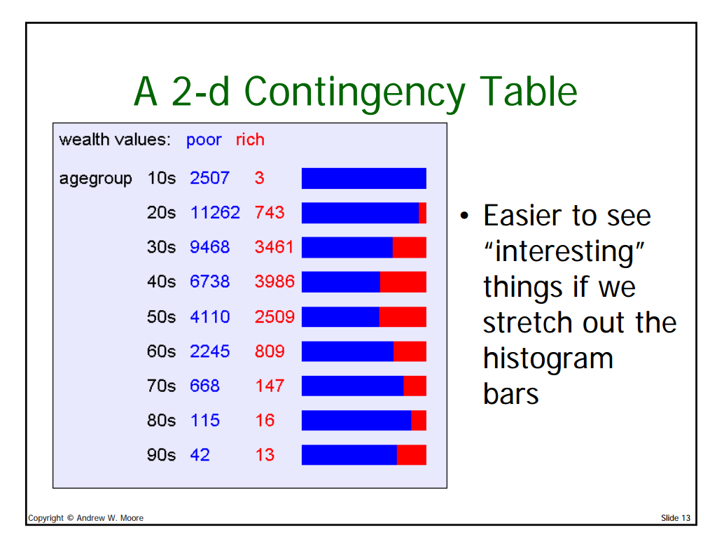
Now this is stretching out the entire histogram graphs.

Online Analytical Processing

Database terminology that I recollect hearing in the stanford db-class.org. It was reserved as the last part of the database class.

Software packages can view slices (the term, first I heard in bangalore office) and aggregates of database table.

Why would people want to look at Contigency Tables?

They want to get a full picture view and understand the word from multiple dimensions.

With n attributes, how many m-d contingency tables are there?

There are n choose m contingency tables.

With 100 attributes, how may 3-d contingency tables are there?

\[100 C_{3} = (100 * 99 * 98) / (3 * 2 * 1) = 161700\]

Data Mining

Data mining is the process of finding patterns in the data. Things like which patterns are interesting, which could merely be illusions and how can they be exploited.

Which patterns are interesting?

The answer will turn out be the engine that drives the decision tree learning.

Information theory

Another generic term and it is broad topic. It was used with data compression, but it is now used in data mining too. The topic of Information Gain forms a sub-part of this topic.

You are trying to predict, if it is easy to ask computer to find which attribute has the highest information gain?

• From this slide, I did not understand, H(wealth), H(wealth|relation) and IG (wealth| relation). What are they?

Learning Decision Trees

Learning Decision Trees is a tree structured plan of set of attributes to test in order to predict the output.

To decide which attribute should be tested first, simply find the one with highest information gain, test it and then recurse. (At this point, what is the clear definition of Information Gain?)

A Decision Stump

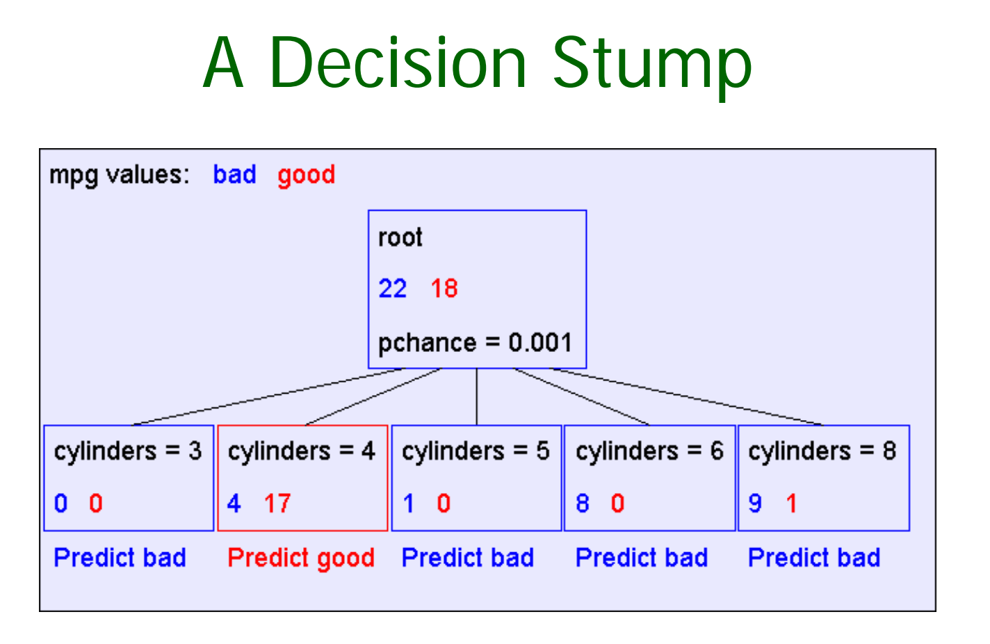
• What is pchance here ?
• How did we come with 22 and 18 as values.

The final tree

You have to follow the tree to understand the various decision that could be taken after asking about the particular value.

Base cases for recursion

• If all records have same output or all records cannot be subdivided using some other attribute, then do not recurse.
• Intuitively, this is proposing another base case, which states that if there is no information gain, then do not recurse.

• But there is a problem with that theory. The example is that of X-OR gate.

Basic Decision Tree summarized

Reference Slides

• Weka Tutorial

Lecture Notes

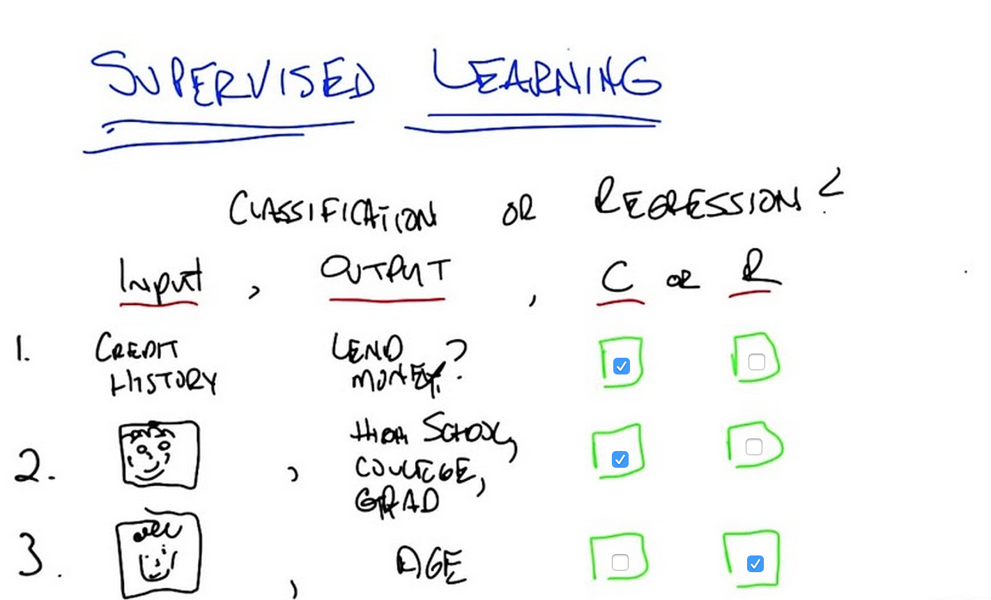
Difference between classification and regression

scribble

slides

transcript

C: Today we are going to talk about supervised learning. But, in particular what we’re going to talk about are two kinds of supervised learning, and one particular way to do supervised learning. Okay, so the two types of supervised learning that we typically think about are classification and regression. And we’re going to spend most of the time today talking about classification and more time next time talking about regression. So the difference between classification and regression is fairly simple for the purposes of this discussion. Classification is simply the process of taking some kind of input, let’s call it x. And I’m going to define these terms in a couple of minutes. And mapping it to some discrete label. Usually, for what we’re talking about, something like, true or false. So, what’s a good example of that? Imagine that I have a nice little picture of Michael.So what do you think, Michael? Do you think this is a male or a female?

M: So you’re, you’re classifying me as male or female based on the picture of me and I would think you know, based on how I look I’m clearly male.

C: Yes. In fact, manly male. So, this would be a classification from pictures to male. And this is where we’re going to spend most of our time talking about it first as a classification task. So taking some kind of input, in this case pictures, and mapping it to some discrete number of labels, true or false, male or female, car versus cougar, anything that, that you might imagine thinking of.

M: Car versus cougar?

C: Yes. Okay, so that’s classification. We’ll return to regression in a little bit later during this conversation. But, just as a preview, regression is more about continuous value function. So, something like giving a bunch of points. I want to give in a new point. I want to map it to some real value. So we may pretend that these are examples of a line and so given a point here, I might say the output is right there. Okay, so that’s regression but we’ll talk about that in a moment. Right now, what I want to talk about is classification.

M: Would an example of regression also be, for example, mapping the pictures of me to the length of my hair? Like a number that represents the length of my hair?

C: Absolutely, for the purposes of the sort of things that we’re going to be worried about you can really think of the difference between classification and regression is the difference between mapping from some input to some small number of discrete values which might represent concepts. And regression is mapping from some input space to some real number. Potentially infinite number of real numbers.

Supervised Learning Quiz

scribble

slides

transcript

M: Alright, so, let’s see what happened here. So, what you’re saying is in some cases the inputs are discrete or continuous or complicated. In other cases the outputs could be discrete or continuous or complicated. But I think what you were saying is what matters to determine if something is classification or regression is whether the output is from a discrete small set or whether it’s some continuous quantity. Is that right?

C: Right, that’s exactly right. The difference between a classification task or a regression task is not about the input, it’s about the output. If the output is continuous then it’s regression and if the output is small discrete set or discrete set, then it is a classification task. So, with that in mind, what do you think is the answer to the first one?

M: So, lend money. If it was something like predicting a credit score, that seems like a more continuous quantity. But this is just a yes no, so that’s a discrete class, so I’m going to go with classification.

C: That is, correct. It is classification and the short answer is, because it’s a binary task. True, false. Yes, no. Lend money or don’t lend money. So it’s a simple classification test. Okay, with that in mind, what about number two?

M: Alright, so number two. It’s trying to judge something about where they fall on a scale, high school, college, or grad student. But all of, the system is being asked to do is put them into one of those three categories, and these categories are like classes, so it’s classification.

C: That is also exactly right. Classification. We moved from binary to trinary in this case, but the important thing is that it’s discrete. So it doesn’t matter if it’s high school, college grad, professor, elementary school, any number of other ways we might decide where your status of matriculation is a small discrete set. So, with that in mind, what about number three?

M: Alright, so the input is the same in this case. And the output is kind of the same except there’s, well there’s certainly more categories because there’s more possible ages than just those three. But when you gave the example you did explicitly say that ages can be fractional like, you know, 22.3. So that definitely makes me think that it’s continuous, so it should be regression.

C: Right, I think that is exactly the right thing, you have a continuous output. Now, I do want to point something out. That while the right answer is regression, a lot of people might have decided that the answer was classification. So, what’s an argument? If I told you in fact the answer was classification, what would be your argument for why that would be?

M: I mean, you know, if you think about ages as being discrete. You just say, you know, you can one or two or three or, you know, whatever up to set. There isn’t really, you know, usually we don’t talk about fractional ages. So it seems like you could think of it as a set of classes.

C: Right. So let’s imagine. So, how old are people? Let’s imagine we only cared about years, so you’re either one or two or three or four or five. Or maybe you can be one and a half, and two and a half, and three and a half. But, whatever, it’s, it’s not all possible real number values. And we know that people don’t live beyond, say, 250. Well, in that case, you’ve got a very large discrete set but it’s still discrete. Doesn’t matter whether there’s two things in your set, three things in your set, or in this case 250 things in your set, it’s still discrete. So, whether it’s regression, or classification,depends upon exactly how you define your output and these things become important. I’m going to argue that in practice, if you were going to set up this problem, the easiest way to do it would be to think about it as a real number and you would predict something like 23.7. And so it’s going to end up being a regression task and we can might, maybe think about that a little bit more as we move along. So either answer would be acceptable depending upon what your explanation of exactly what the output was. You buy that?

M: That makes sense.

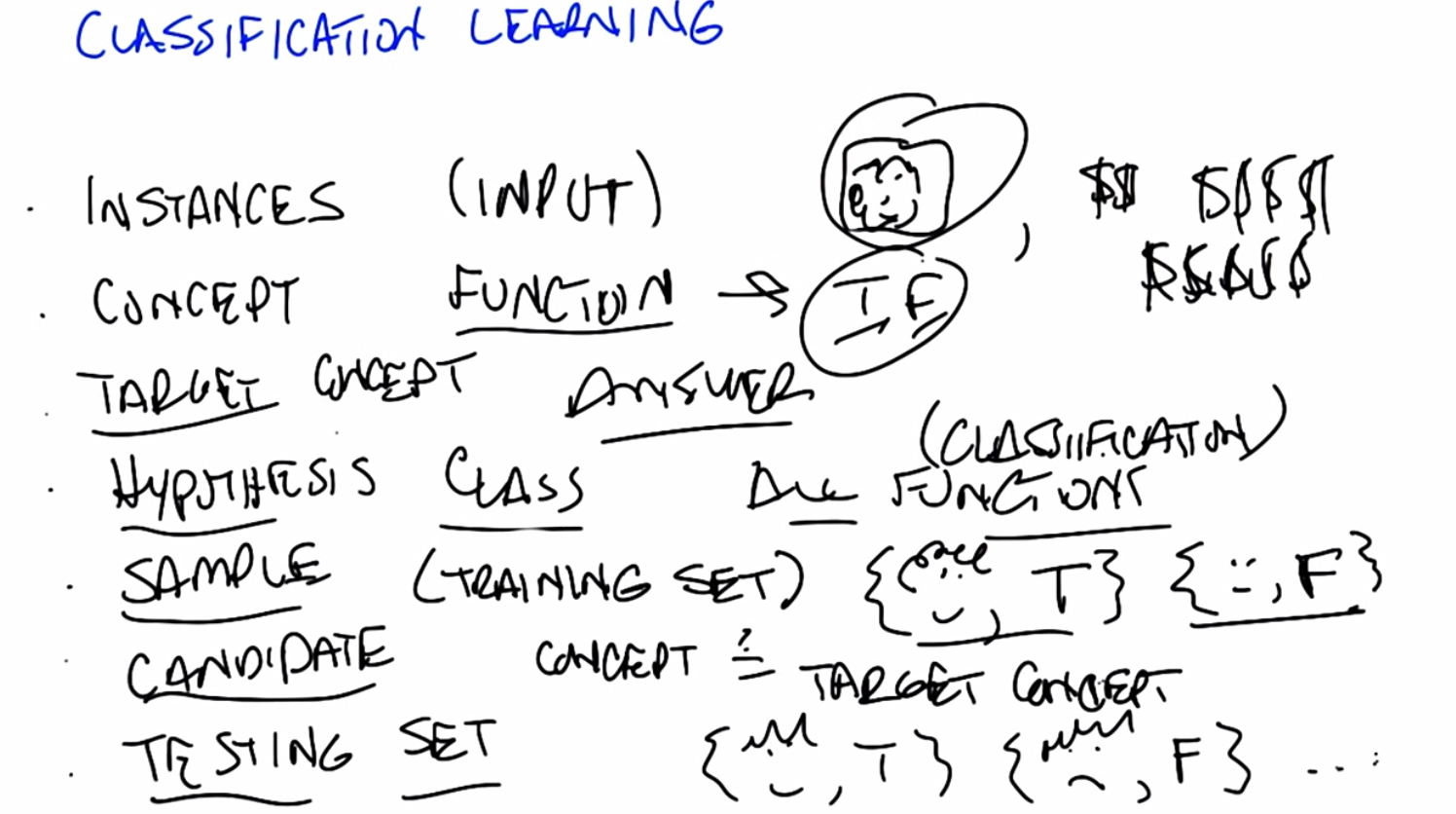
Classification Learning

scribble

• target concept is the thing we are trying to find.

slides

transcript

C: Before we get into the details of that, I want to define a couple of terms. Because we’re going to be throwing these terms out all throughout the lessons. And I want to make certain that we’re all on the same page and we mean the same thing. But we’re returning to this again and again and again. So, the first term I want to introduce is the notion of instances. So, instances, or another way of thinking about them is input. Those are vectors of values, of attributes. That define whatever your input space is. So they can be pictures and all the pixels that make up pictures like we’ve been doing so far before. They can be credit score examples like how much money I make, or how much money Michael makes. So whatever your input value is, whatever it is you’re using to describe the input, whether it’s pixels or its discrete values, those are your instances, the set of things that you’re looking at. So you have instances, that’s the set of inputs that you have. And then what we’re trying to find is some kind of function and that is the concept that we care about. And this function actually maps inputs to outputs, so it takes the instances, it maps them in this case to some kind of output such as true or false. This is the, the categories of things that we’re worried about. And for most of the conversation that we’re going to be having, we’re going to be thinking about binary classification, just true and false. But the truth is, this would work whether there were three outputs, as we did with high school, college, or grad school, or whether there were 250 as we were contemplating for ages. But the main thing here is the concept, is the function that we care about that’s going to map pictures, for example true or false.

M: So okay, I get, I get the use of the word,” instance”, right?” Instance” is just, like, a single thing that’s out there. But I have an intuitive notion of what a concept is. How does that relate to this more formal notion? Like, can we connect this to the intuitive notion of what a concept is?

C: I guess so. So a concept, I don’t know. How would you want to put that? So a concept is something that, I mean were talking about is a notion of a function, so what it means formally is that you have some input, like a picture, and it immediately inputs maps anything in that input space to some particular defined output space, like true or false, or male or female, or credit worthy or not. Intuitively a concept is an idea describes a set of things. OK, so we can talk about maleness or femaleness. We can talk about short and tall; we can talk about college students and grad students. And so the concept is the notion of what creditworthiness is, what a male is, what a college student is.

M: Okay, I think I see that. So essentially if you want to think about the concept of tallness, one way to define it is to say, Well in general if you give me something I can tell you rather or not its tall so it’s going to map those somethings to am I tall or not. True or false.

C: Right, exactly and so really when you think about any concept and we talk about this in generally AI is effectively a way of saying is effectively a set of things. That are apart of that concept. So, you can have a concept of a car and if I gave you “cars” you would say these things are in it and if I gave you “non-cars” you would say they are not. And so a concept is, therefore by definition, a mapping between objects in a world and membership in a set, which makes it a function.

C: So with that, with that notion of a concept as functions or as mappings from objects to membership in a set we have a particular target concept. And the only difference between a target concept and the general notion of concept is that the target concept is the thing we’re trying to find. It’s the actual answer. So, a function that determines whether something is a car or not, or male or not, is the target concept. Now this is actually important, right, because we could say that. We have this notion in our head of things that are cars or things that are males, or thing, or people who are credit worthy but unless we actually have it written down somewhere we don’t know whether it’s right or wrong. So there is some target concept we’re trying to get of all the concepts that might map pictures or people to true and false. M: Okay, so if you trying to teach me what tallness is so you have this kind of concept in mind of these, these things are tall and these things are not tall. So you’re going to have to somehow convey that to me. So how are you going to teach me?

C: Well that’s what comes up with the rest of these things that we’re defining here. So let me tell you what the next four things are then you can tell me whether that answers your question. M: Got it. C: OK, so we’ve got a notion of instances, input, we’ve got a notion of concepts. Which take input and maps into some kind of output. And we’ve got the sum target constant, some specific function, some particular idea that we’re trying to find, we’re trying to represent. But out of what? So that’s where the hypothesis comes in. And in fact I think it’s better to say hypothesis class. So that’s the set of all concepts that you’re willing to entertain. So it’s all the functions I’m willing to think about. M: So why wouldn’t it just be all possible functions?

C: It could be all possible functions and that’s a perfectly reasonable hypothesis class. The problem with that is that if it is all possible functions it may be very, very hard for you. Figure out which function is the right one given finite data. So when we actually go over decision trees next I think it will be kind of clear why you need to pick a specific hypothesis class. So let’s return to that in a little bit but it’s an excellent question. So, conceptually in the back of your head until we, we come to specific examples, you can think of hypothesis class as simply being all possible functions in the world. On the other hand, even so far just the classification learning, we already know that we’re restricting ourselves to a subset of all possible functions in the world, because all possible functions in the world includes things like x squared, and that’s regression. And we’ve already said, we’re not doing regression. So already hypothesis classes all functions we care about and maybe it’s all classification functions. So we’ve already picked a subset. So we got all these incidences, got all these concepts, we want to find a particular concept and we’ve got this set of functions we’re willing to look at. So how are we going to determine what the right answer is. So if you try to answer Michael’s question that we do that in machine learning is with a sample or another name for which I prefer is a training set.

Classification Learning 3

scribble

• classification based on data, which is inductive learning.

slides

transcript

C: So what’s a training set? Well a training set is a set of all of our inputs, like pictures of people, paired with a label, which is the correct output. So in this case, yes, this person is credit worthy.

M: You can tell I’m creditworthy based on my curly hair.

C: Versus someone who has no curly hair and therefore is obviously not creditworthy. And if you get bunches and bunches of examples of input and output pairs, that’s a training set. And that’s what’s going to be the basis for you figuring out what is the correct concept or function.

M: I see. So instead of just telling me what tall means, you’re going to give me lots of examples of, this is tall, this is not tall, this is tall, this is not tall. And that’s the way that you’re explaining what the target concept is.

C: Right. So if you want to think about this in the real world, it’s as if we’re walking down the street and I’m pointing out cars to you, and non-cars to you, rather than trying to give you a dictionary that defines exactly what a car is. And that is fundamentally inductive learning as we talked about before. Lots and lots of examples, lots of labels. Now I have to generalize beyond that. So, last few things that we we talk about, last two terms I want to introduce are candidate, and testing set. So what’s a candidate? Well a candidate is just simply the, a concept that you think might be the target concept. So, for example, I might have, right now, you already did this where you said, oh, okay I see, clearly I’m creditworthy because I have curly hair. So, you’ve effectively asserted a particular function that looks at, looks for curly hair, and says, if there’s curly hair there, the person’s credit worthy. Which is certainly how I think about it. And people who are not curly hair, or do not have curly hair are, in fact, not creditworthy. So, that’s your target concept. And so, then, the question is, given that you have a bunch of examples, and you have a particular candidate or a candidate concept, how do you know whether you are right or wrong? How do you know whether it’s a good candidate or not? And that’s where the testing set comes in. So a testing set looks just like a training set. So here our training set, we’ll have pictures and whether someone turns out to be creditworthy or not. And I will take your candidate concept and I’ll determine whether it does a good job or not, by looking at the testing set. So in this case, because you decided curly hair matters, I have drawn, I have given you two examples from a training set, both of which have curly hair, but only one of which is deemed credit worthy. Which means your target concept is probably not right.

M: So to do that test I, guess you can go through all the pictures in the testing set, apply the candidate concept to see whether it says true or false, and then compare that to what the testing set actually says that answer is.

C: Right, and that’ll give you an error. So by the way, the true target concept is whether you smile or not.

M: Oh. That does make somebody credit-worthy.

C: It does in my world. Or at least I, wish it did in my world. Okay. So, by the way an important point is that the training set and the testing set should not be the same. If you learn from your training set, and I test you only on your training set, then that’s considered cheating in the machine learning world. Because then you haven’t really shown the ability to generalize. So typically we want the testing set set to include lots of examples that you don’t see in your training set. And that is proof that you’re able to generalize.

M: I see. So, like, if you’re a teacher and you’re telling me, you give me a bunch of fact and then you test me exactly on those facts, I don’t have to have understood them. I just can regurgitate them back. If you really want to see if I got the right concept, you have to see whether or not I can apply that concept in new examples.

C: Yes, which is exactly why our final exams are written the way that they are written. Because you can argue that I’ve learned something by doing memorization, but the truth is you haven’t. You’ve just memorized but here you have to do generalization. As you remember from our last discussion, generalization is the whole point of machine learning.

Example 1 - Dating

scribble

slides

transcript

C: All right, so we’ve defined our terms, we know what it takes to do at least supervised learning. So now I want to do a specific algorithm and a specific representation, that allows us to solve the problem of going from instances to, actual concepts. So what we’re going to talk about next are decision trees. And I think the best way to introduce decision trees is through an example. So, here’s the very simple example I want you to think about for a while. You’re on a date with someone. And you come to a restaurant. And you’re going to try to decide whether to enter the restaurant or not. So your input, your instances are going to be features about the restaurant. And we’ll talk a little bit about what those features might be. And the output is whether you should enter or not. Okay, so it’s a very simple, straightforward problem but there are a lot of details here that we have to figure out.

M: It’s a classification problem.

C: It’s clearly a classification problem because the output is yes, we should enter or no, we should move on to the next restaurant. So in fact, it’s not just a classification problem, it’s those binary classification problems that I said that we’d almost exclusively be thinking about for the next few minutes. Okay. So, you understand the problem set up? M: Yes, though I’m not sure exactly what the pieces of the input are.

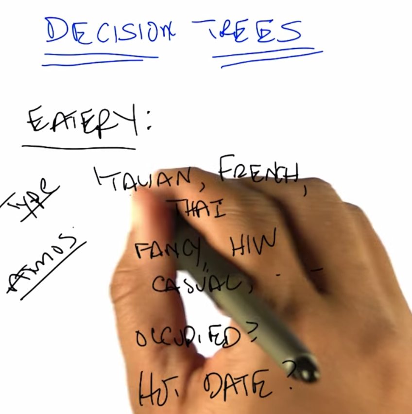
C: Right, so thats actually the right next question to ask. We have to actually be specific now about a representation. Before I was drawing squiggly little lines and you could imagine what they were, but now since we’re really going to go through an example, we need to be clear about what is it mean to be standing in front of the restaurant. So, let’s try to figure out how we would represent that, how we would define that. We’re talking about, you’re standing in front of a restaurant or eatery because I can’t see the reliably small restaurant. And we’re going to try to figure out whether we’re going to go in or not. But, what do we have to describe our eatery? What do we have? What are our attributes? What are the instances actually made of? So what are the features that we need to pay attention to that are going to help us to determine whether we should yes, enter into the restaurant. Or no, move on to the next restaurant. So, any ideas Michael?

M: Sure. I guess there’s like the type of restaurant.

C: Okay, let’s call that the type. So it could be Italian, it could be French, it could be Thai, it could be American, there are American restaurants, right? M: Sure.

C: Greek, it can be, Armenian. It can any kind of restaurant you want to. Okay, good. So that’s something that probably matters because maybe you don’t like Italian food or maybe you’re really in the mood for Thai. Sounds perfect. Okay anything else? M: Sure. How about whether it smells good?

C: You know, I like cleanliness. Let’s be nice to our eateries and let’s say atmosphere. So is it fancy? Is it a hole-in-the-wall? Those sorts of things. You could imagine lots of things like that, but these things might matter to you and your date. Okay, so, we know the type of the restaurant that we have, we know whether it’s fancy, whether it’s casual, whether it’s a hole in the wall. Some of the best food I’ve ever had are in you know, well-known hole in the walls. Those sorts of things. Anything else you can think of?

M: Sure, Sometimes, I might like looking inside and seeing whether there’s people in there and whether they look they’re having a good time.

C: Right. So that’s an important thing. So let’s just say if it’s occupied. Now why might that matter in reality? Well it matters because if it’s completely full and you may have to wait for a very long time, you might not want to go in. On the other hand. If you’re looking at a restaurant you’ve never heard of, and there’s only two people in it, and it’s Friday at 7 p.m. Maybe that says something about something. Maybe you want it to be quiet. You know, those sorts of things might matter. Okay, so we’ve got atmosphere, we’ve got occupied. Anything else you can think of?

M: I have been out of the dating market for a while, but I guess how hard I am trying to work to impress my date.

C: Perfect. So do you have a hot date or not? Or, this is someone who you really, really, really want to impress and so, maybe it matters then, it’s even more important whether it’s a fancy restaurant or a hole in the wall, or whether it’s French or whether it’s an American restaurant. Notice, by the way, that the first two sets that we have have multiple possible categories here. So it could be Italian, French, Thai, American, so on and so forth. Atmosphere is something that can have many, many possible values, but the last two things that we talked about were all binary. Either it’s occupied or it’s not. Yes or no or, you have a hot date or you don’t. And I think we could go on like this for a long time but, let’s try to move on to maybe a couple of other features and then try to actually figure out how we may actually solve this.

Representation

scribble

slides

transcript

C: Alright, so Michael. Last set of features that that’s come up with three or four, three or four more features and then move on.

M: Sure. So come up with a couple. Alright, so I could, sometimes I’ll look at the menu that’s posted outside, and I’ll see if the, you know? How pricey it is. Okay, so cost. Right, so cost can be represented as discrete input. By the way, it could also be represented as an actual number. Right? We could say, look it’s cheap, it’s moderately expensive, it’s really expensive or you could have a number which is the average cost of an entry. And it doesn’t really matter for, for what we’re talking about now but just some way of representing cost.

C: Okay. Just give me one or two more features but I want to give me some features that don’t have anything to do with the restaurant itself but might still be important.

M: So, whether I’m hungry?

C: I like that. Here’s another one. What’s the weather like. Is it raining outside? Which is a different sense of atmosphere because if it’s raining outside, maybe it’s not your favorite choice but you don’t want to walk anymore. Okay, so we have a ton of features here. We’ve gone through a few of them. Notice that some of the specifically have to do with the restaurant and some of them have to do with things that are external to the restaurant itself but you can imagine that they’re all important. Or possibly important to whether you should enter into the restaurant or not. Agreed? And there’s a bunch of features you could imagine coming up with that probably have nothing to do with whether you should enter into the restaurant or not. Like, how many cars are currently parked across the country. Probably doesn’t have an impact on whether you’re going to enter into a specific restaurant or not. Okay. So, we have a whole bunch of features and right now we’re sticking with features we think that might be relevant. And we’re going to use those to make some kind of decision. So, that gets us to decision trees. So, the first thing, that, that we want to do is, we want to separate out what a decision tree is from the algorithm that you might use to build the decision tree. So the first thing we want to think about is the fact that a decision tree has a specific representation. Then only after we understand that representation and go through an example, we’ll start thinking about an algorithm for finding or building a decision tree. Okay, so a decision tree is a very simple thing. Well, you might be, might be surprised to know it’s a tree, the first part of it. And it looks kind of like this. So, what I’ve drawn for you is example. Sample generic, decision tree. And what you’ll see is three parts to it. The first thing you’ll see is a circle. These are called nodes, and these are in fact, decision nodes. So, what you do here, is you pick a particular attribute and you ask a question about it. The answer to that question, which is its value for what the edges represent in your tree. Okay. So we have these nodes which represent attributes, and we have edges which represent value. So let’s be specific about what that means. So here’s a particular attribute we might pick for the top node here. Let’s call it hungry. That’s one of the features that Michael came up with. Am I hungry or not? And there’s only two possible answers for that. yes, I’m hungry, true, or false, I am not hungry. And each of these nodes represent some attribute. And the edges represent the answers for specific values. So it’s as if I’m making a bunch of decisions by asking a series of questions. Am I hungry? And if the answer is yes, I am hungry, then I go and I ask a different question. Like is it rainy outside? And maybe it is rainy and maybe it’s not rainy, and let’s say if it isn’t rainy then I want to make a decision, and so these square boxes here are the actual output. Okay so you’re hungry, yes, and it’s not raining, so what do you do? So, let’s just say you go in. True, I go in so, when it’s, I’m hungry and it’s not raining, I go in.

M: That truth is answering a different question. It’s not in the nodes I guess. So, in the leaves, the t and f means something different.

C: That’s right. It’s the out, that’s exactly right. The, the leaves, the little boxes, the leaves of your decision tree is your answer. What’s on the on the edges are the possible values that your attribute can take on. So, in fact, let’s try to, let’s make that clear by picking a different by picking another possible attribute. You could imagine that if I am not hungry, what’s going to matter a lot now is say, the type of restaurant, right. Which we said there were many, many types of restaurants. So if I’m not hungry, then what matters a lot more is the type of restaurant, and so I’ll move down this path instead and start asking other questions. But ultimately what this decision tree allows me to do is to ask a series of questions and depending upon those answers, move down the tree, until eventually I have some particular output answer, yes I go in the restaurant, or no I do not.

Quiz on Representation

scribble

slides

transcript

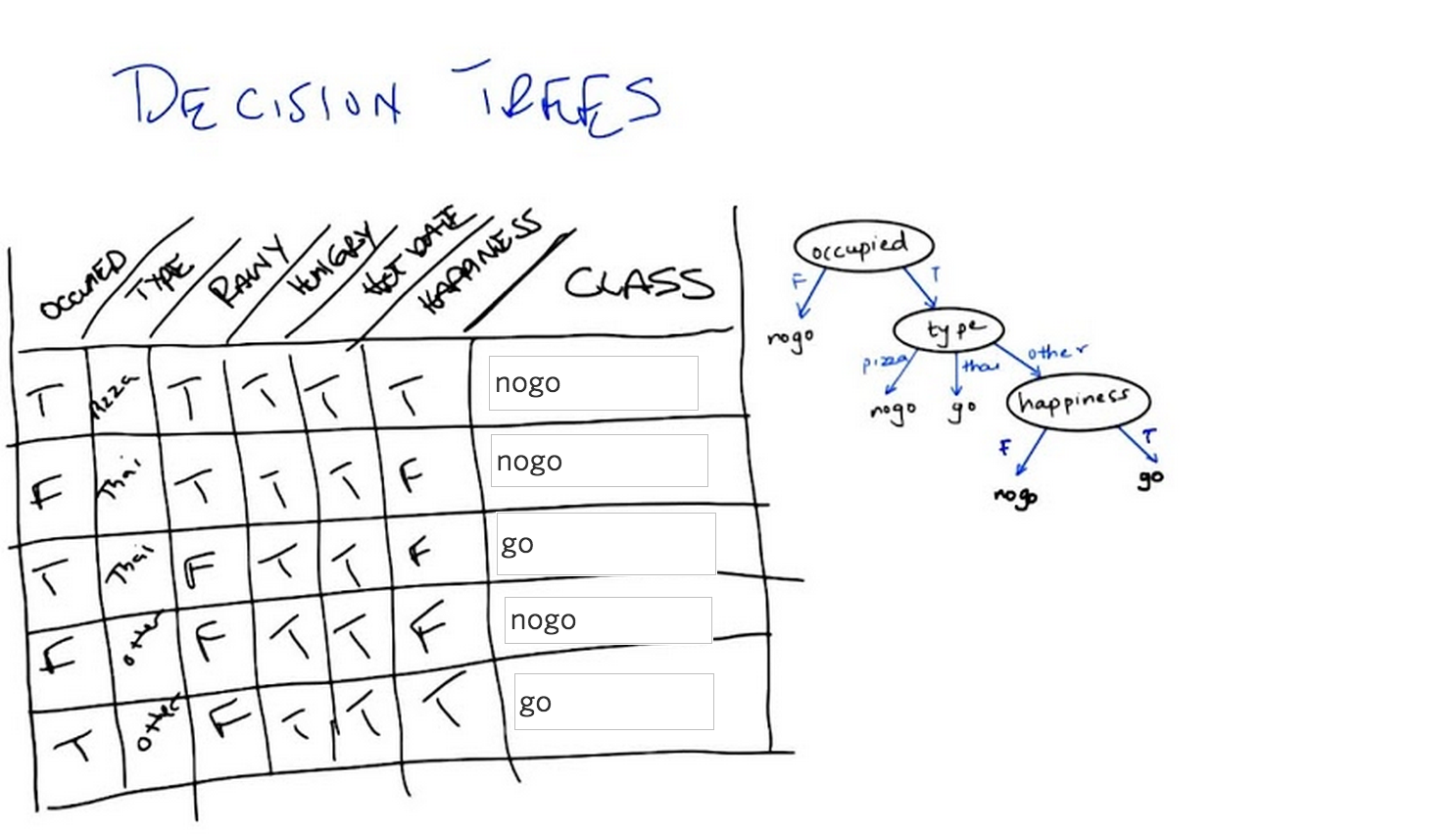
Okay, so we’ve now seen an abstract example of decision trees. So let’s make certain that we understand it with a concrete example. So, to your right is a specific decision tree that looks at some of the features that we talked about. Whether you are occupied or not, whether the restaurant is occupied or not what type of restaurant it is. Your choices are pizza, Thai, or other. And whether the people inside look happy or not. The possible outputs are again binary either you don’t go or you do go, into the restaurant. On your left is a table which has six of the features that we’ve talked about. Whether the restaurant is occupied or not, the type of restaurant, whether it’s raining outside or not, whether you’re hungry or not. Whether you’re on a hot date and whether the people inside look happy, and some values for each of those. And what we would like for you to do is to tell us what the output of this decision tree would be in each case. Each row of this is a different time that we’re stopping at a restaurant, and the, the little values there summarize what is true about this particular situation. And, and you’re saying we need to then trace through this decision tree and figure out what class is.

answer

C: Now the nice thing about a decision tree sort of conceptually and intuitively, is that it really is asking a series of questions. So, we can simply look at these rows over here and the values that our features have and we can just follow down the path of the tree. So, in the first case. We have true. We have true for occupied, which means we want to go down the right side of the tree. And check on the type. So in the first case, the type is pizza. And so we go down the first branch and that means. We do not go down the tree. So, the output is no go.

M: So, okay, so now, I got a different answer. So, I looked at this and I said happiness is true. And, the bottom box says happiness true, you go.

C:Right. So, you got that wrong, you got what I’m going to tell you is the wrong answer by going from the bottom of the tree up. The way decision trees work is you always start at the root of the tree. That is the very top of the tree. And you ask the questions in that order. If you start at the bottom, you can’t go up.

M: So I’ll do the second instance. The second instance, you say that we need to start at the top of the tree where it says occupied. And so now I look at the instance and the instance says that it’s false for occupied, so we go down that left branch and we hit no go. Oh wait but now I haven’t look at any of the other nodes.

C: You don’t have to look at any of the other nodes because it turns out that if it’s not occupied you just don’t go into a restaurant. So you’re the type of person who doesn’t like to be the only person in a restaurant. So that’s a no-go. That’s an important point, Michael. Actually, you might also notice that this whole tree, even if you look at every single feature in the tree, only has three of the attributes. It only looks at occupied. Type and happiness.

M: I see. So hot date is sort of irrelevant which is good, because in this case it’s not really changing from instance to instance anyway.

C: True. And neither is hungry you might notice. Although raining does in fact change a little bit here and there. But it apparently it doesn’t matter.

M: Because you always take an umbrella.

C: Got it. Okay, so let’s quickly do the other three and see if we we come to the same conclusion.

M: Alright. Well all the instances that have occupied false we know those are no go, right away. So we can do it kind of out of order. And the other ones are both occupied. One is tie and one is other. For the tie one we go. The other one, oh I see, for the other one we have to look at whether there’s happiness or not, and in this instance happiness is true. So we get on the right branch and we go.

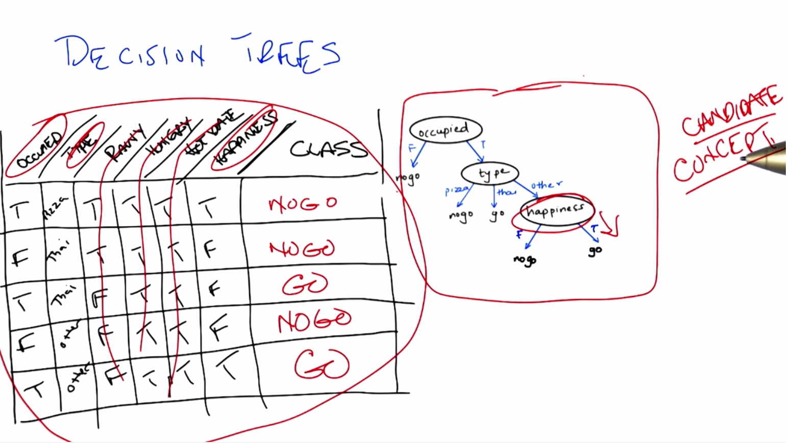
C: Exactly it. So we notice hot date doesn’t matter, hungry doesn’t matter and rainy doesn’t matter. And the only thing that matters are whether you’re occupied, what type of restaurant you’re at and whether you’re happy or not. Or whether the, the patrons in the restaurants are restaurant is, are happy or not. But, here’s the other thing about this. It’s not just about the features. Let’s tie it back in to the other things, that we mentioned in the beginning. This, in our case, this table actually represents our testing set. It’s the thing that we’re going to look at to determine whether we were right or wrong. These are the examples that we’re going to do to see whether we generalize or not. And this particular tree here is our candidate concept. So there’s lots and lots and lots of other trees that we might have used. We might have used a tree that also took, asked questions about whether it was rainy or not or asked questions about whether you were on a hot date or not. But we didn’t. We picked a specific tree that had only these three features and only asked in this particular way. So what we’re going to talk about next. Is how we might decide whether to choose this tree over any of the other possible number of trees that we might have chosen instead.

Quiz: Best Attribute

scribble

slides

Prior concept discussion slide

transcript

C: Alright, so let’s take a moment to have a quiz where we really delve deeply into what it means to have a best attribute. So something Michael and I have been throwing around that term, let’s see if we can define it a little bit more crisply. So, what you have in front of you are three different attributes that we might apply in our decision tree for sorting out our instances. So, at the top of the screen what you have is you have a cloud of instances. They are labelled either with red x or a green o, and that represents the label so that means that they are part of our training set, so this is what we’re using to build and to learn our Decision Tree. So, in the first case you have the set of instances being sorted into two piles. There are some xs and some os on the left and some xs and some os on the right. And the second case you have that same set of data being sorted so that all of it goes to the left and none of it goes to the right. And in the third case you have that same set of data that’s sorted so that a bunch of the xs end up on the left and a bunch of the os end up on the right. What I want you to do is to rank each one, where one is the best and three is the least best attribute to choose. Go.

answer

M: So, did you say one was the best.

C: One is the best and three is the least best.

M: Alright, so I am really excited about the third cloud structure. The third attribute to be split on. Because what it does is it takes all our x’s and o’s that need to have different labels and it puts them into two different buckets. One where they all get to be red x’s and the other where they all get to be green o’s. So I would say the far right one is ranked number one.

C: I would agree with you and in fact I would say that we’re done.

M: Yeah, it’s perfect.

C: It is perfect, agreed. One is perfect. Or 3 is perfect in this case, because I gave it a one.

M: Alright, so then, I think the worst one is also easy to pick, because if you look at the middle attribute, the attribute that’s shown in the middle, we take all the data, and we put it all on the left. So we really have just kicked the can down the road a little bit. There’s nothing this attribute splitting has done. So, I would call that the worst possible thing you could do. Which is to basically to do nothing.

C: Okay. So what about the first attribute?

M: So this one is sort of in between that it splits things so you have smaller sets of data to deal with, but it hasn’t really improved our ability to tell the reds and the greens apart. So in fact, I’d almost want to put this as three also but I’ll put it as two. Okay. I think an argument could be making it three.

C: An argument could be made for making it two. Your point is actually pretty good, right? We have eight red things and eight green things up here. And the kind of distribution between them, sort of half red and, half red x’s, half green o’s, we have the same distribution after we go through this attribute here. So it does some splitting, but it’s still, well you still end up with half red, half green, half x, half o. So, that’s not a lot of help, but it’s certainly better than doing absolutely nothing.

M: Well is it though? I mean, it seems it could also be the case. That what we’ve done is that we’re now splitting on that has provided no valid information, and therefore can only contribute to overfitting.

C: Do you want to change your answer? I would accept either two or a three as an answer here. I think you can make an argument either way. And I think you actually made both arguments.

Decision Tree Expressiveness

scribble

slides

transcript

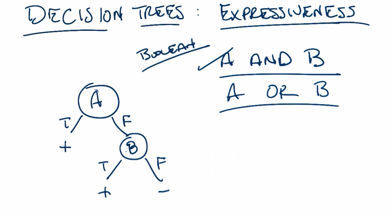
C: So, we saw before when we looked at AND and OR versus XOR that in the case of AND and OR we only needed two nodes but in the case of XOR we needed three. The difference between two and three is not that big, but it actually does turn out to be big if you start thinking about having more than simply two attributes. So, let’s look at generalized versions of OR and generalized versions of XOR and see if we can see how the size of the decision tree grows differently. So in the case of an n version of OR. That is we have n attributes as opposed to just two. We might call that the any function. That is a function where any of the variables are true then the output is true. We can see that the decision tree for that has a very particular and kind of interesting form. Any ideas Michael about what that decision tree looks like?

M: So, well. So going off of the way you described OR in the two case. We can start with that. And you. You pick one of the variables. And if its true then yeah. Any of them is true since the leaf is true.

C: What happens if its false?

M: Well, then we have to check what everything that’s left. So then we move on to one of the other attributes like A2 and again, if it’s true, it’s true and if it’s false then we don’t know. This could take some time.

C: Oh that was actually an interesting point. Let’s say if there were only three, we would be done. But wait, what if there were five?

M: Then we need one more node.

C: What if there were n?

M: Then we need n minus 4 more nodes.

C: Right, so what you end up with in this case is a nice little structure around the decision tree. And how many nodes do we need?

M: Looks like one for each attribute, so that would be n.

C: n nodes, exactly right. So we have a term for this sort of thing, the size of the decision tree is, in fact, linear. In n. And that’s for any. Now what about an n version of XOR?

M: So XOR is, if one is true but the other one’s not true then it’s true. And if they’re both true. Yeah I don’t. It’s not clear how to generalize that.

C: So, while the usual general version of this we like to think of as parity. All parity is a way of counting, so there’s usual two forms of parity that we worry about. Either even parity or odd parity. So let’s pick one, it doesn’t matter. Let’s say odd and all that works out to be in this case is, if the number of attributes that are true is an odd number, then the output of the function is true, otherwise it’s false. Okay, so, how would we make that decision tree work?

M: Ooh. Well, we got to split on something and there all the same, so let’s split on A1 again. So what do we do if A1 is true, versus being false.

M: We don’t know much if A1 is true. We have to look at everybody else.

C: Right. So let’s look at A2. What if A2 is true versus false?

M: Well if A1 and A2 are true then, then the output is going to be whatever the parity of all the remaining variables are. So you still have to do that.

C: Uh-huh, yup. And I’m already running out of room, so let’s pretend there’s only three variables. What’s the output?

M: All right, so the far left. Is there’s three trues which is odd so the output is true. The next leaf over, only two trues. A1 is true, A2 is true, but A3 is false, so that’s two trues which is is even so the answer’s false. Is this pattern continuing? Now we’ve got. No, so then it’s false again because we’ve got two trues and a false to get to the next leaf. And we’ve got one true to get to the next leaf so that’s true. Oh, that looks like XOR.

C: It looks just like XOR. In fact, each one of these sub trees is kind of a version of XOR isn’t it? Now what we have is, we have to do the same thing on the right. So we gotta redo A2, and we’re going to be in the same situation before. And we’re going to start drawing on top of each other.

M: So, what’s the answer to the one on the very right. Where all of them are false.

C: So that’s an even number of trues. Zero is even. So that’s false. Okay, so in the case where only A3 is true, it’s true and we just keep going on and on and on again. Now imagine what would happen, in fact let me ask you Michael, what would happen if we had four attributes instead of three.

M: We get a whole another, a whole other level of this tree.

C: Yep. We have it just goes on and on and on and nobody wants to think about it anymore. So, how many nodes do you think there are?

M: Well, for three there was one, two, three, four, five, six, seven. Which seems suspiciously like one less than the power of two.

C: Mm-hm. And that is exactly right. You need more or less 2 to the n nodes. Or 2 to the n, maybe, minus 1. So let’s just say big O of 2 to the n. Everyone watching this is a computer scientist so they know what they’re doing. Okay so, you need an exponential therefore, as opposed to linear number of nodes. So very quickly you run out of room here. You very, very quickly have a really big tree because it’s growing exponentially. So, XOR is an exponential problem and is also known as hard. Whereas OR, at least in terms of space that you need, it’s a relatively easy one. This is linear. We have another name for exponential and that is evil. Evil, evil, evil. And it’s evil because it’s a very difficult problem. There is no clever way to pick the right attributes in order to give you an answer. You have to look at every single thing. That’s what make this kind of problem difficult. So, just as a general point, Michael, I want to make, is that we hope that in our machine learning problems we’re looking at things that are more like any than we are looking at things that are more like parity because otherwise, we’re going to need to ask a lot of questions in order to answer the, the parity questions. And we can’t be particularly clever about how we do it.

M: Though, if we were kind of clever and added another attribute, which is like, the sum of all the other attribute values, that would make it not so bad again. So maybe it’s just a kind of, bad way of writing the problem down.

C: Well, you know, what they say about AI is that the hardest problem is coming up with a good representation. So what you just did is, you came up with a better representation, where you created some new pair, new variable. Let’s call it B, which is just the sum of all of the As, where we pretend that I don’t know, true is one and false is zero. This is actually a really good idea. It’s also called cheating because you got to solve the problem by picking the best representation in the first place. But you know what? It’s a good point, that in order for a machine running to work, you either need an easy problem or you need to find a clever way of cheating.

Decision Tree Expressiveness

scribble

slides

transcript

C: All right, so what that last little exercise showed is that XOR, in XOR parody, is hard. It’s exponential. But that kind of provides us a little bit of a hint, right? We know that XOR is hard and we know that OR is easy. At least in terms of the number of nodes you need, right? But, we don’t know, going in, what a particular function is. So we never know whether the decision tree that we’re going to have to build is going to be an easy one. That is something linear, say. Or a hard one, something that’s exponential. So this brings me to a key question that I want to ask, which is, exactly how expressive is a decision tree. And this is what I really mean by this. Not just what kind of functions it kind of represent. But, if we’re going to be searching over all possible decision trees in order to find the right one, how many decision trees do we have to worry about to look at? So, let’s go back and look at, take the XOR case again and just speak more generally. Let’s imagine that we once again, we have n attributes. Here’s my question to you, Michael. How many decision trees are there? And look, I’m going to make it easy for you, Michael. They’re not just attributes, they’re Boolean attributes. And they’re not just Boolean attributes, but the output is also Boolean. Got it?

M: Sure. But how many trees? So it’s, I’m going to go with a lot.

C: Okay. A lot. Define a lot.

M: So, alright, well, there’s n choices for which node to split on first. And then, for each of those, there’s n minus 1 to split on next. So I feel like that could be an n factorial kind of thing. And then, even after we’ve done all that, then we have an exponential number of leaves. And for each of those leaves, we could fill in either true or false. So it’s going to be exponential in that too. So you said we have to pick each attribute at every level. And so you see something that you think is probably going to be, you know? Some kind of commutatorial question here. So, let’s say n factorial, and that’s going to just build the nodes. That’s just the nodes. Well, once you have the nodes, you still have to figure out the answers. And so, this is exponential because factorial is exponential. And this is also exponential. Huh. So let’s see if we can write that down. So let me propose a way to think about this. You’re exactly right the way you’re thinking. So, let’s see if we can be a little bit more concrete about it. So, we have Boolean inputs and we have Boolean outputs, so this is just like AND, it’s just like OR, it’s just like XOR, so, whenever we’re dealing with Boolean functions, we can write down a truth table. So let’s think about what the truth table looks like in this case.

C: Alright, so, let’s look at the truth table. So what a truth table will give me is, for, the way a truth table normally works is you write out, each of the attributes. So, attribute one, attribute two, attribute three, and dot dot dot. And there’s n of those, okay? We did this a little earlier. When we did our decision tree. When we tried to figure out whether I was on a hot date or not. And then you have some kind of output or answer. So, each of these attributes could take on true or false. So one kind of input that we may get would be say all trues. Right? But we also might get all trues, except for one false at the end. Or maybe the first one’s false and all the rest of them are true, and so on, and so forth. And each one of those possibilities is another row in our table. And that can just go on for we don’t know how long. So we have any number of rows here and my question to you is how many rows? Go.

answer

C: What’s the answer Michael? How many rows do we have? M: So if it was just one variable we’re splitting on, then it need to be true or false, so, that’s two rows. If it was two variables, then there’s four combinations and three, would be eight, combinations. So, generalizing the end, it ought to be 2 to the n.

C: That’s exactly right, there are 2 to the n different rows. And, that’s what always happen when we’re dealing with n, you know, n attributes, n boolean attributes. There’s always 2 to the n possibility. Okay, so I get just halfway there and I get to your point about, combinatorial choices, among the attributes but that’s only the number of rows that we have. There’s another question ,we need to ask which is, exactly how big is the truth table itself?

ID3

scribble

• We choose the best attribute as the one which gives the maximum gain.

slides

transcript

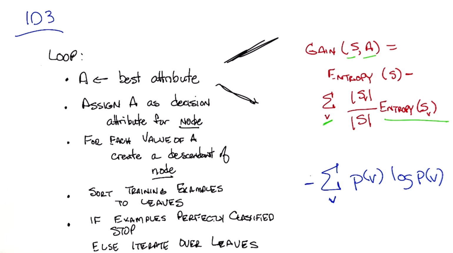
So now, we have an intuition of best, and how we want to split. We’ve, we’ve looked over, Michael’s proposed, the high-level algorithm for how we would build a decision tree. And I think we have enough information now that we can actually do, a real specific algorithm. So, let’s write that down. And the particular algorithm that Michael proposed is a kind of generic version of something that’s called ID3. So let me write down what that algorithm is, and we can talk about it. Okay, so here’s the ID3 algorithm. You’re simply going to keep looping forever until you’ve solved the problem. At each step, you’re going to pick the best attribute, and we’re going to define what we mean by best. There are a couple of different ways we might define best in a moment. And then, given the best attribute that splits the data the way that we want, it does all those things that we talked about, assign that as a decision attribute for node. And then for each value that the attribute A can take on, create a descendent of node. Sort the training examples to those leaves based upon exactly what values they take on, and if you’ve perfectly classified your training set, then you stop. Otherwise, you iterate over each of those leaves, picking the best attribute in turn for the training examples that were sorted into that leaf, and you keep doing that. Building up the tree until you’re done. So that’s the ID3 algorithm. And the key bit that we have to expand upon in this case, is exactly what it means to have a best attribute. All right, what exactly is it that we mean by best attribute? So, there are lots of possibilities, that you can come up with. The one that is most common, and the one I want you to think about the most, is what’s called information gain. So information gain is simply a mathematical way to capture the amount of information that i want to gain by picking particular attribute. But what it really talks about is the reduction in the randomness, over the labels that you have with set of data, based upon the knowing the value of particular attribute. So the formula’s simply this. The information gain over S and A where S is the collection of training examples that you’re looking at. And A, as a particular attribute, is simply defined as the entropy, with respect to the labels, of the set of training examples, you have S, minus, sort of, the expected or average entropy that you would have over each set of examples that you have with a particular value.

M: So what we’re doing, we’re picking an attribute and that attribute could have a bunch of different values, like true or false, or short, medium, tall?

C: Right and that’s represented by v.

M: Okay, each of those is a different v. And then we’re saying okay, for over those leaves, we’re going to do this entropy thing again and we are right. So what is entropy?

C: So, we’ll talk about entropy later on in the class in some detail and define it exactly and mathematically. And some of you probably already know, what entropy is, but for those of you who don’t, it’s exactly a measure of randomness. So if I have a coin, let’s say a two-headed coin. It can be heads or tails, and I don’t know anything about the coin except that it’s probably fair. If I were to flip the coin, what’s the probability that it would end up heads or tails?

M: A half.

C: It’s a half, exactly, if it’s a fair coin it’s a half. Which means that I have no basis, going into flipping the coin, to guess either way whether it’s heads or it’s tails. And so that has a lot of entropy. In fact it has exactly what’s called one bit of entropy. On the other hand, let’s imagine that I have a coin that has heads on both sides. Then, before I even flip the coin, I already know what the outcome’s going to be. It’s going to come up heads. So what’s the probability of it coming up with heads?

M: It’s one.

C: So that actually has no information, no randomness, no entropy whatsoever. And has zero bits of entropy. So, when I look at this set of examples that I have, and the set of labels I have, I can count the number that are coming up, lets say, red x’s. Versus the ones that are coming up green o’s. And if those are evenly split, then the entropy of them is maximal, because if I were to close my eyes and reach for an instance, I have no way of knowing beforehand whether I’m more likely to get an x or I’m more likely to get an o. On the other hand, if I have all the x’s in together, then I already know before I even reach in that I’m going to end up with an x. So as I have more of one label than the other the amount of entropy goes down. That is I have more information going in. Does that make sense, Michael?

M: I think so can we say what the formula is for this or not?

C: Sure. What is the formula for it? You should remember.

M: I’m not sure what the notation ought to be with these

S’s but it has something to do with P(log)P.

C: So the actual formula for entropy, using the same notation that we’re using for information game is simply the sum, over all the possible values that you might see, of the probability of you seeing that value, times the log of the probability of you seeing that value, times minus one. And I don’t want to get into the details here. We’re going to go into a lot more details about this later when we get further on in the class with randomize optimization, where entropy’s going to matter a lot. But for now, I just, you have, I want you to have the intuition that this is a measure of information. This is the measure of randomness in some variable that you haven’t seen. It’s the likelihood of you already knowing what you’re going to get if you close your eyes and pick one of the training examples, versus you not knowing what you’re going to get. If you close your eyes and you picked one of the training examples. Okay?

M: Alright. So, well, so, okay, so then in the practice, trees that you had given us before, it was the case that we worked, we wanted to prefer splits that I guess, made things less random, right? So if things were all mixed together, the reds and the greens, after the split if it was all reds on one side and all greens on the other. Then each of those two sides would have what? They would have very low entropy, even though when we started out before the split we had high entropy.

C: Right, that’s exactly right. So if you remember the three examples before. One of them, it was the case that all of the samples went down the left side of the tree. So the amount of entropy that we had, didn’t change at all. So there was no gain in using that attribute. In another case, we split the data in half. But in each case, we had half of the x’s and half of the o’s together, on both sides of the split. Which means that the total amount of entropy actually didn’t change at all. Even though we split the data. And in the final case, the best one, we still split the data in half, but since all of the x’s ended up on one side and all of the o’s ended up on the other side, we had to entropy or no randomness left whatsoever. And that gave us the maximum amount of information gain.

M: So is that how we’re choosing the best attribute? The one with the maximum gain?

C: Exactly. So the goal is to maximize over the entropy gain. And that’s the best attribute.

ID3 Bias

scribble

slides

transcript

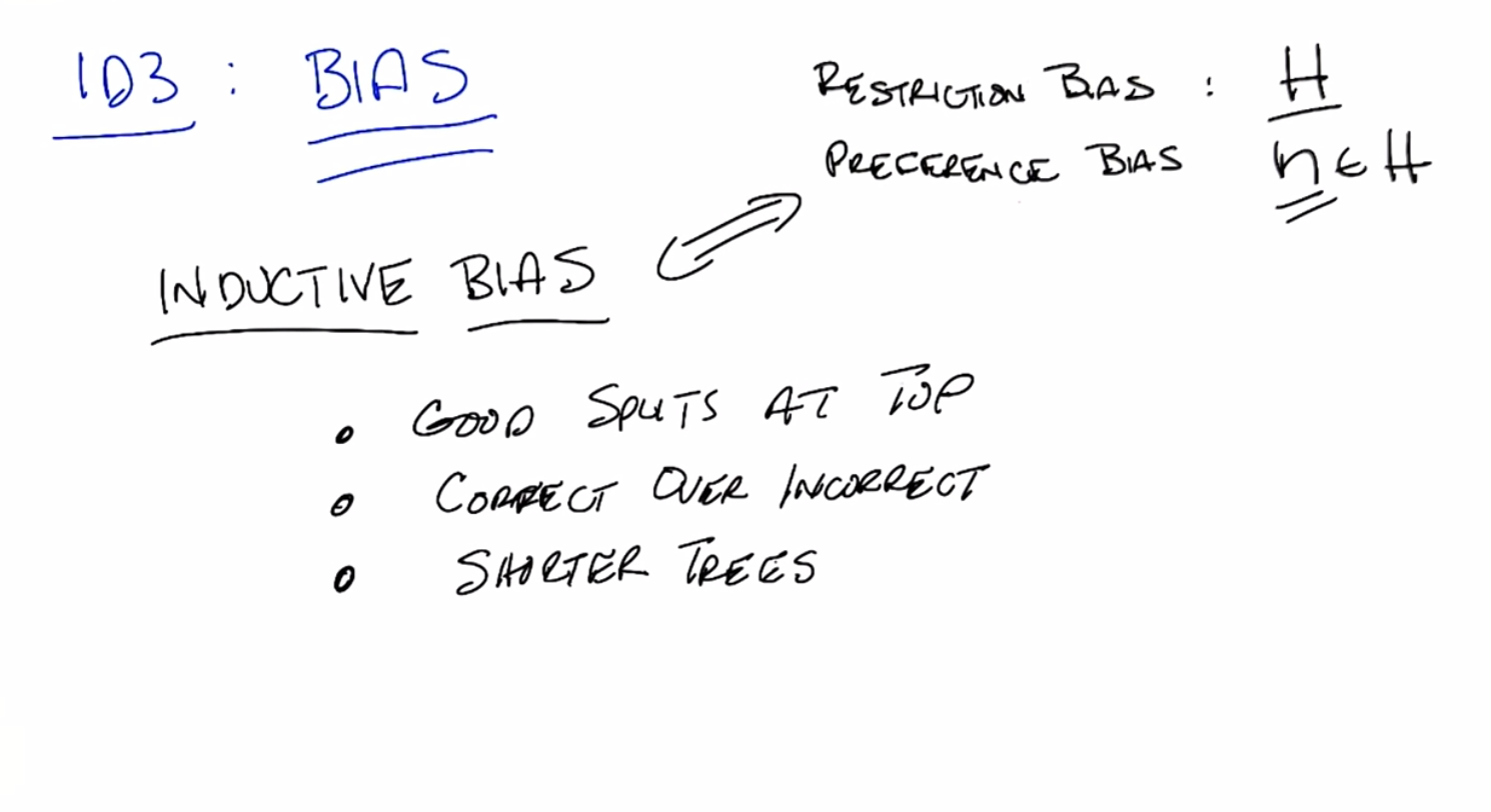
C: So, we’ve got a whole bunch of trees we have to look at, Michael. And were going to have to come up with some clever way to look through them. And this get’s us back, something that we’ve talked about before, which is the notion of bias. And in particular, the notion of inductive bias. Now, just as a quick refresher, I’m want to remind you that there is two kind of biases we worrying about when we think about algorithms that are searching through space. One is what’s called a restriction bias. The other is called preference bias. So a restriction bias is nothing more than the hypothesis set that you actually care about. So in this case, with the decision trees, the hypothesis set is all possible decision trees. Okay? That means we’re not considering, y equals 2x plus non-boolean functions of a certain type. We’re only considering decision trees, and all that they can represent. And nothing else. Okay? So that’s already a restriction bias and it’s important. Because, instead of looking at the infinite number uncountably infinite number of functions that are out there, that we might consider. We’re only going to consider those that can be represented by a decision tree over in, you know, all the cases we’ve given so far discrete variable. But a preference bias is something that’s just as important. And it tells us what source of hypotheses from this hypothesis set we prefer, and that is really at the heart of inductive bias. So Michael, given that, what would you say is the inductive bias of the ID3 algorithm? That is, given a whole bunch of decision trees, which decision trees would ID3 prefer, over others?

M: So, it definitely tries, since it’s, since it’s making it’s decisions top down. It’s going to be more likely to produce a tree that has basically good splits near the top than a tree that has bad splits at the top. Even if the two trees can represent the same function.

C: Good point. So good splits near the top. Alright. And you said something very important there Michael. Given two decision trees that are both correct. They both represent the function that we might care about. It would prefer the one that had the better split near the top. Okay, so any other preferences? Any other inductive bias on the ID3 algorithm.

M: It prefers ones that model the data better to ones that model the data worse.

C: Right. So this is one that people often forget: it prefers correct ones to incorrect ones. So, given a tree that has very good splits at the top but produces the wrong answer. It will not take that one over one that doesn’t have as good splits at the top, but does give you the correct answer. So that’s really, those are really the two main things that are the inductive bias for ID3. Although, when you put those two together, in particular when you look at the first one, there’s sort of a third one that comes out as well, which is ID3 algorithm tends to prefer shorter trees to longer trees. Now, that preference for shorter trees actually comes naturally from the fact that you’re doing good splits at the top. Because you’re going to take trees that actually separate the data well by labels, you’re going to tend to come to the answer faster than you would if you didn’t do that. So, if you go back to the example where we went before, where one of the attributes doesn’t split the data at all, that is not something that ID3 would go for, and it would in fact create a longer and unnecessarily longer tree. So it tends to prefer shorter trees over longer trees. So long as they’re correct and they give you good splits near the top of the tree.

Decision Trees Continuous Attributes

scribble

• This is for dealing with continuous attributes.
• We have to learn from the training set as what attributes we should split over.

slides

transcript

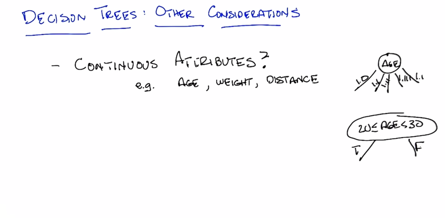
C: Alright. So, we’ve actually done pretty well. So through all of this, we finally figured out what decision trees actually are. We know what they represent. We know how expressive they are. We have an algorithm that lets us build the decision trees in an effective way. We’ve done just about everything there is to do with decision trees, but there is still a couple of open questions that I want to think about. So, here’s a couple of them and I want you to, to think about and then we’ll discuss them. So, so far all of our examples that we’ve used. All the the things we’ve been thinking about for good pedagogical reasons. We had not only discreet outputs but we also had discrete inputs. So one question we might ask ourselves, is what happens if we have, continuous attributes? So Michael, let me ask you this. Let’s say we had some continuous attributes. We weren’t just asking whether someone’s an animal or whether they’re human or whether it’s raining outside or we really cared about age or weight or distance or anything else that might have a continuous attribute. How are we going to make that work in a decision tree?

M: Well, I guess the literal way to do it would be for something like age to have a branching factor that’s equal to the number of possible ages.

C: Okay, so that’s one, one possibility. So we stick in age and then we have one. 1.0, we have one for 1.1, we have one for 1.11, we have one for 1.111

M: Ahh, I see. Alright. Well, at the very least, okay. What if, what if we only included ages that were in the training set? Presumably there’s at least a finite number of those. Oh, we could do that. We could just do that, except what are we going to do then when we come up with something in the future that wasn’t in the training session.

M: Oh, right. Can we look at the testing set?

C: No were not allowed to look at the testing set. That is cheating, and not the kind of good cheating that we do when we pick a good representation.

M: Okay, fair enough. Well we could, we could do ranges. What about ranges? Isn’t that the way we cover more than just individual values?

C: Give me an example. Say ages you know, in the 20s.

M: Okay, so, huh. How would we represent that with a decision tree? You could do like age, element sign, bracket. 20, 21, or 29 or 30 right per end.

C: Yeah it’s too much. Why don’t I just say age is between or less is, let’s see, greater than or equal to, 20 and, less than 30. And just draw a big oval for that. Alright? So that’s a range, so that’s all numbers between, 20 and 30 inclusive of 20 but not 30 right and what’s good about that is that’s a question.

M: So, I guess the good news there is that now we know how to evaluate attributes like that because we have a formula from three that tells you what to do but seems like there’s an awful lot of different ones to check.

C: Right, and in fact if it’s truly a continuous variable, there are in principal an infinite number of them checked. But we can do now the sort of cheating you wanted to do before. We can just look at the training set, and we could try to pick questions that cover the sorts of data in the training set. So, for example, if all of the values are in the 20s, then there is no point of even asking the question. You will start just instead splitting upon values that were, say less than where you might do that. You might look at all of the values that show up in the training set, and say well, I am going to do a binary search. So, I am just going to create an attribute for Less than half of whatever is in the training set or greater than half of whatever the range is in the training set. Does that make sense?

M: Yeah, that’s clever.

C: Right. Thank you. I just made that up on the spot. Okay, so you do those sorts of things and that’s how you would deal with continuous attributes.

Quiz: Decision Trees Other Consideration

scribble

slides

transcript

So, here’s the next question I want to ask you, simple true or false question. Does it make sense to repeat an attribute along any given path in the tree? So, if you we pick some attribute like A, should we ever ask a question about A again? Now, I mean something very specific about, by that. I mean, down a particular path of the tree, not just anywhere else in the tree. So, in particular, I mean this. So, I ask a question about A, then I ask a question about B, and then I ask a question about A again. That’s the question I’m asking. Not whether A might appear more than once in the tree. So, for example, you might have been the case where A shows up more than once in the tree, but not along the same path. So, in the second case over here, A shows up more than once, but they really don’t really have anything to do with one another because once you’ve answered B, you will only ever ask the question about A once. So, my question to you is, does it make sense to repeat A more than once along a particular path in the tree? Yes or No.

answer

M: So, alright. Does it make sense to repeat, an attribute along a path in the tree? So, it seems like it could be no point in that, you know, if we’re looking at attributes like, you know, is a true, then later we would ask again is a true because we would already have known the answer to that.

C: Right, and by the way, information gain will pick that for you automatically.

M: It doesn’t have to be a special thing in the algorithm if you consider an attribute that you’ve already split on, then you’re not going to gain any information, so it’s going to be the worst thing, to split on. But it seems like maybe you’re trying to lead us on because we’re in the continuous attributes portion of our show.

C: Okay, well what’s the answer there? Is the answer not also false?

M: Well we wouldn’t want to ask the same question, about the same attribute. So, we wouldn’t have age between 20 and 30, and then later ask age so we might have a different range, on age later in the tree.

C: So, that’s exactly right, Michael. So, the answer is no, it does not make sense ,to repeat an attribute along a path of the tree, for discrete, value trees. However, for continuous valued attributes, it does make sense. Because, what you’re actually doing, is asking a different question. So, one way to think about this, is that the question is age in the 20’s or not. Is actually a discrete valued attribute that you’ve just created, for the purposes of the decision tree. So, asking that question doesn’t make sense but asking a different question, about age, does in fact make sense. So once you know that you are not in the 20’s you might ask well am I less than 20 years old? Maybe a teenager or am I greater than 40. How old am I, 44? Greater than 44, in which case, I’m old.

Decision Trees Other Considerations

scribble

• We get really really good at generalizing the data, but it does not help us with generalizing. This is called as over fitting.
• Pruning is an effective way to deal with over fitting.
• It is a simple addition to ID3 algorithm.

slides

transcript

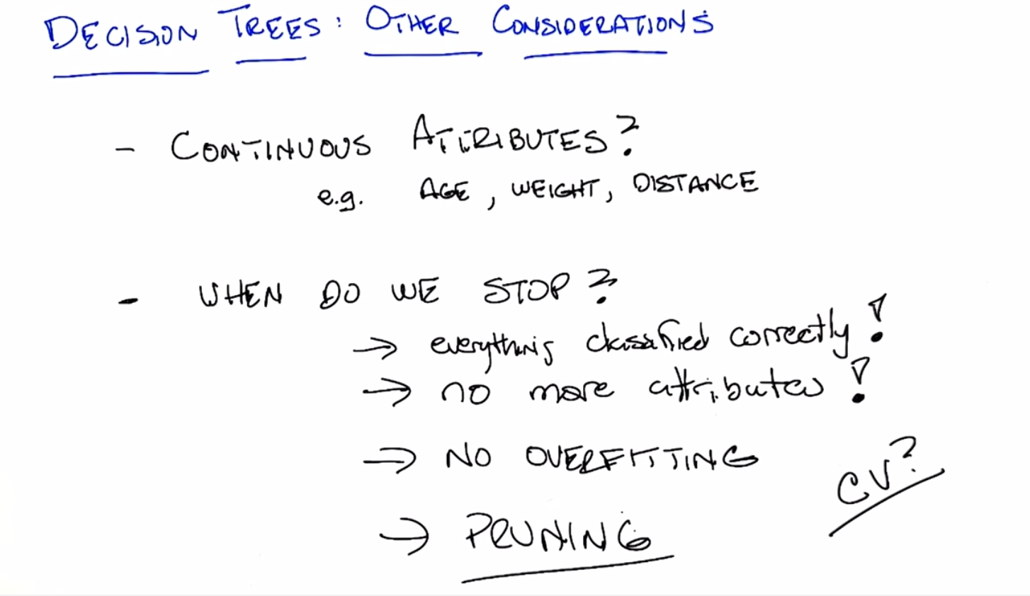
C: So, we’ve answered the thing about continuous attributes. Now, here’s another thing. When do we really stop?

M: When we get all the answers right. When all the training examples are in the right category class.

C: Right, so the the answer in the algorithm is when everything is classified correctly. That’s a pretty good answer, Michael. But what if we have noise in our data? What if it’s the case that we have two examples of the same object, the same instance, but they have two different labels? Then this will never be the case.

M: Oh. So, then our algorithm goes into an infinite loop.

C: Which seems like a bad idea.

M: So we could just say, or we’ve run out of attributes.

C: Or we’ve run out of attributes. That’s one way of doing it. In fact that what’s going to have to happen at some point, right? That’s probably a slightly better answer. Although that doesn’t help us in the case where we have continuous attributes and we might ask an infinite number of questions. So we probably need a slightly better criteria. Don’t you think?

M: So, what got us down this path, was thinking about what happens if we have noise. Why would we be worried about having noise anyway?

C: Well, I guess the training data might have gotten corrupted a little bit or maybe somebody copied something down wrong.

M: Right, so since that’s always a possibility, does it really make sense to trust the data completely, and go all the way to the point where we perfectly classify the training data? But Charles, if we can’t trust our data, what can we trust?

C: Well, we can trust our data, but we want to verify. The whole point is generalization. And if it’s possible for us to have a little bit of noise in the data, an error here or there, then we want to have some way to deal to handle that possibility, right?

M: I guess so.

C: I mean, we actually have a name for this, right? When you get really, really, really good at classifying your training data, but it doesn’t help you to generalize, we have a name for that.

M: Right. That sounds like overfitting.

C: Exactly. We have to worry about overfitting. Okay, step one, have a different personality with maximal information gain. Okay, so we don’t want to, we don’t want to overfit. So we need to come up with some way of overfitting. Now the way you overfit in a decision tree is basically by having a tree that’s too big, it’s too complicated. All right. Violates Occam’s Razor. So, what’s a kind of, let’s say, modification to something like ID3 to our decision tree algorithm that will help us to avoid overfitting?

M: Well last time we talked about overfitting, we said cross-validation was a good way of dealing with it, which, it allowed us to choose from among the different, say degrees of the polynomial. So maybe we could do something like that? I don’t know. Try all the different trees and, see which one has the lowest cross validation error? Maybe there’s too many trees.

C: Maybe, but that’s a perfectly reasonable thing to do, right? You take out a validation set. You build a decision tree, and you test it on the validation set and you pick whichever one has the lowest error in the validation sect, that’s one way to avoid it. And then you have, don’t have to worry about this question about stopping, you just grow the tree on the training set minus the validation set until it does well on that. And you check it against the cross valid, you check it against the validation set, and you pick the best one. That’s one way of doing it, and that would work perfectly fine. There is another way you can do it that’s more efficient. Which is, you do the same idea validation, except that you hold out a set and every time you decide whether to expand the tree or not, you check to see how this would do so far in the validation set. And if the error is low enough, then you stop expanding the tree. That’s one way of doing it. M: So is there, is there a problem in terms of, I mean if we’re expanding the tree depth for search wise, we could be at, you know, we could be looking at one tiny little split on one side of the tree before we even look at any, anything on the other side of the tree.

C: That’s a fine point. So how would you fix that?

M: Maybe expand breadth first?

C: Yeah, that would probably do it. Anything else you could think of? Well, so, you could do pruning, right? You could go ahead and do the tree as if you didn’t have to worry about over-fitting, and once you have the full tree built, you could then do a kind of, you could do pruning. You could go to the leaves of the tree and say, well, what if I collapse these leaves back up into the tree? How does that create error on my validation set? And if the error is too big, then you don’t do it. And if it’s very small, then you go ahead and do it. And that should help you with overfitting. So, that whole class of ways of doing it, is called pruning. And there’s a whole bunch of different ways you might prune. But pruning, itself, is one way of dealing with overfitting, and giving you a smaller tree. And it’s a very simple addition to the standard ID3 algorithm.

Decision Trees. Other Considerations Regression

scribble

slides

transcript

C: So another consideration we might want to think about with decision trees but you’re not going to go into a lot of detail but I think might be worth at least mentioning is the problem of regression. So, so far we’ve only been doing classification where the outputs are discrete, but what if we were trying to solve something that looked more like x squared or two x plus 17 or some other continuous function. In other words, a regression problem. How would we have to adapt decision trees to do that? Any ideas Michael?

M: So these are now continuous outputs, not just continuous inputs.

C: Right, maybe the outputs are all continuous, maybe the outputs are discrete, maybe they’re a mix of both.

M: Well it certainly seems like out rule of using, information gain is going to run into trouble because it’s not really clear how you measure information on these continuous values. So, I guess you could measure error some other way. Well it’s not error, it’s trying to measure how mixed up things are? Oh so ,maybe something like variance? Cause in a continuous space you could talk about if there’s a big spread in the values that would be measured by the variance.

C: Oh good. So what you really have now is a question about splitting. What’s the splitting criteria?

M: I guess there’s also an issue of what you do in the leaves.

C: Right. So, what might you do in the leaves?

M: I guess you could do some sort of more standard kind of fitting algorithm. So, like, report the average or, or do some kind of a linear fit.

C: Is any number of things you can do. By the way ,that’s worth pointing out on the, on the output that if we do pruning like we did before, we have errors, we did actually say when we talked about that how you would report an output. Right? If you don’t have a clear answer where everything is labeled true or everything is labeled false, how do you pick? So something like an average would work there.

M: I don’t know, I mean, it seems like it depends on what we’re trying to measure with the tree. If the tree is, we’re trying to get as many right answers as we can, then you probably want to do like a vote in the leaves.

C: Right, which ,at least, if the only answer is true or false, that would look more like an average I guess. Right, so you pick, you do a vote. So we do a vote, so we do pruning. We do have to deal with this issue of the output. Somehow ,and something like a vote mixing. And here, when you have a regression, then I guess average is a lot like voting.

M: Yeah, in a continuous phase.

C: Yeah. So either way we’re doing a kind of voting. I like that.

Summary of Decision Trees

scribble

• There is lot more and we will learn as we do assignments.
• Concepts were covered in detail at the end of the lesson.

slides

transcript