Ensemble Learning Boosting
scribble
slides
transcript
M: Hey Charles, how’s it goin’?
C: It’s going pretty well Michael. How’s it going with you?
M: Good, thank you.
C: Good, good, good. Guess what we’re going to talk about today?
M: Well, reading off this screen, it looks like maybe ensemble learning, and boosting, whatever that is.
C: Yes, that’s exactly what we’re going to talk about. We’re going to talk about a class of algorithms called ensemble learners. And I think you will see that they’re related to some of the stuff that we’ve been doing already, and in particular we’re going to spend most of our time focusing on boosting because boosting is my favorite of the ensemble learning algorithms. So you ready for that?
M: Yeah! Let’s do it.
C: Okay. So, I want to start this out by going through a little exercise with you. I want you to think about a problem. Okay. And the particular problem I want you to think about is, spam email.
M: Mm, I think about that a lot.
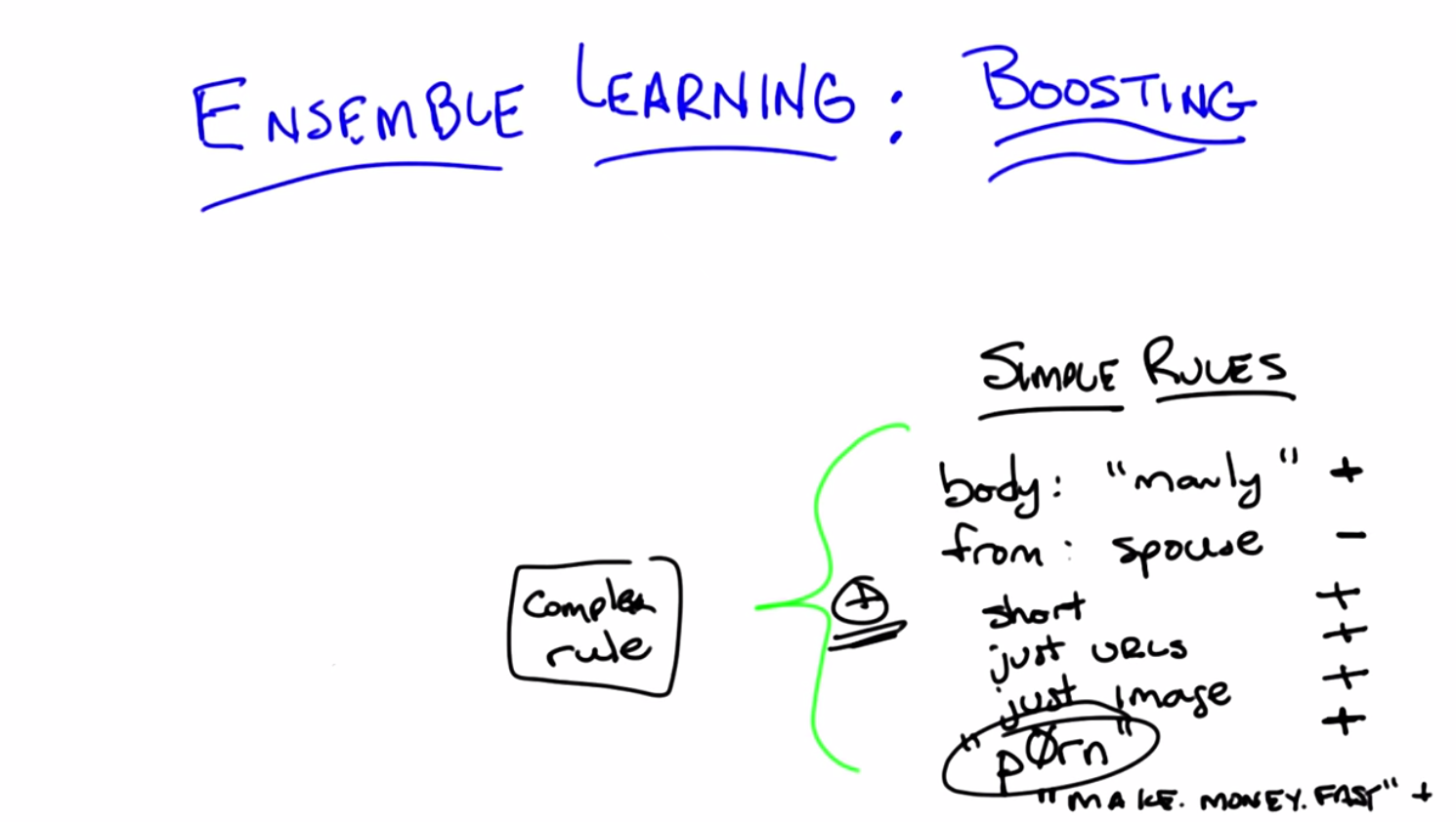
C: So, normally we think of this as a classification task, right, where we’re going to take some email and we’re going to decide if it’s spam or not. Given what we’ve talked about so far, we would be thinking about using a decision tree or, you know, neural networks or k-NN – whatever that means with email. We would be coming up with all of these sort of complicated things. I want to propose an alternative which is going to get us to ensemble learn. OK and here’s the alternative. I don’t want you to try to think of some complicated rule that you might come up with that would capture spam email. Instead, I want you to come up with some simple rules that are indicative of spam email. Okay, so let me be specific, Michael. We have this problem with spam email. That is, you you’re going to get some email message and you want some computer program to figure out automatically for you if something is a piece of spam or it isn’t. And I want you to help write a set of rules that’ll help me to figure that out. And I want you to think about simple rules, so can you think of any simple rules that might indicate that something is spam?
M: Alright I can, yeah I can think of some simple rules. I don’t think they would be very good, but they might be better than nothing. Like if, for example, it mentions how manly I am, I, I would be willing to believe that was a spam message. So like, if the body of the message contains the word manly.
C: Okay, I like that – when the body contains manly. I like that rule, because I often get nonspam messages talking about being manly. So I guess one man’s spam is another man’s normal email.
M: I guess that’s true.
C: Probably. Any other rules?
M: Sure. If it comes from my spouse, it’s probably not spam.
C: OK, so let’s see, from spouse.
M: Her name’s Lisa. Now we’re going to call her our spouse. So we’ll put a minus sign next to “spouse” and a plus sign next to “manly.” So we know some rules are indicative of being spam, and some rules are indicative of not being spam. Okay, anything else?
C: Possibly the length of the message. I guess. Like what?
M: I don’t know. I don’t know that this would be very accurate, but I think some of this, some of the spam I get sometimes is very, very short just like the, it’s like the URL. Like hey, check out this site, and then there’s a URL.
C: Hm, I like that. So, we’ll just say short. Just contains URLs. Hm, I like those rules. Let’s see if we can think of anything else. Oh, how about this one. It’s just an image.
M: Hm.
C: I get a lot of those where it’s just an image.
M: I see, and if you look at the picture it’s all various pharmaceuticals from Canada.
C: Exactly. Here’s one I get a lot.
M: Hm,
C: Lots of misspelled words that you end up reading as being a real word.
M: Hm. But I don’t know how I’d write that as a rule. Or you could just list the words.
C: Like rules that, words that have already been modified in that way. I guess so.
M: Yeah, kind of a, kind of a blacklist, a blacklist of words.
C: Okay so, words like, I would say manly, but you were saying brawn.
M: Or whatever that says. Yeah, so there are tons of these, right? I mean, another one that’s very popular if you’re old enough anyway is this one, remember this one?
C: Oh, sure that was sometimes a virus, right?
M: Yes. Our young, our younger viewers will not know this but this was one of the first big spam messages that would get out there. Make money fast. And there’s tons and tons of these. We could come up with a bunch of them. Now, here’s something they all kind of have in common, Michael, and you’ve touched on this already. All of them are sort of right. They’re useful but no one of them is going to be very good at telling us whether a message has spam on its own. Right. So the word manly is evidence but it’s not enough to decide whether something is spam or not. It’s from your spouse, it’s evidence it’s not spam, but sometimes you get messages from your spouse that are in fact spam, because in fact, she didn’t actually send them. You know, and so on and so forth. And sometimes you get email from princes in Nigeria, and they’re not always spam. I actually do, but any case, sometimes people are asking you for money, and maybe that’s a message you want to ignore, but it isn’t necessarily spam. And some people are very interested in getting messages like this and don’t consider it spam, right?
C: So, so, okay, so I can see that these would all maybe provide some evidence, but it seems really hard to figure out the right way of combining them all together to, I don’t know, make a decision.
M: Right, this is exactly right. And, by the way, if you think about something like decision trees, there’s really a sort of similar problem going on there. We can think of each of the nodes in a decision tree as being a very simple rule and the decision tree tells us how to combine them. Right? So, we need to figure out how to do that here and that is the fundamental notion of ensemble learning.
C: But wait, couldn’t you also do something similar with something like neural networks, where each of these rules becomes a feature and we’re just trying to learn ways to combine them all together. So that would kind of satisfy what you were talking about.
M: True, I mean I think the the difference here in this case and and I think you’re absolutely right but one difference here is that typically with the new network we’ve already built the network itself and the nodes and we’re trying to learn the weights whereas in something like a decision tree you’re building up rules as you go along. And typically with ensemble learning you’re building up a bunch of rules and combining them together until you got something that’s good enough. But you’re absolutely right. You could think of networks as being an ensemble of little parts. Sometimes hard to understand, but an ensemble nonetheless.
Ensemble Learning Simple Rules
scribble
slides

transcript
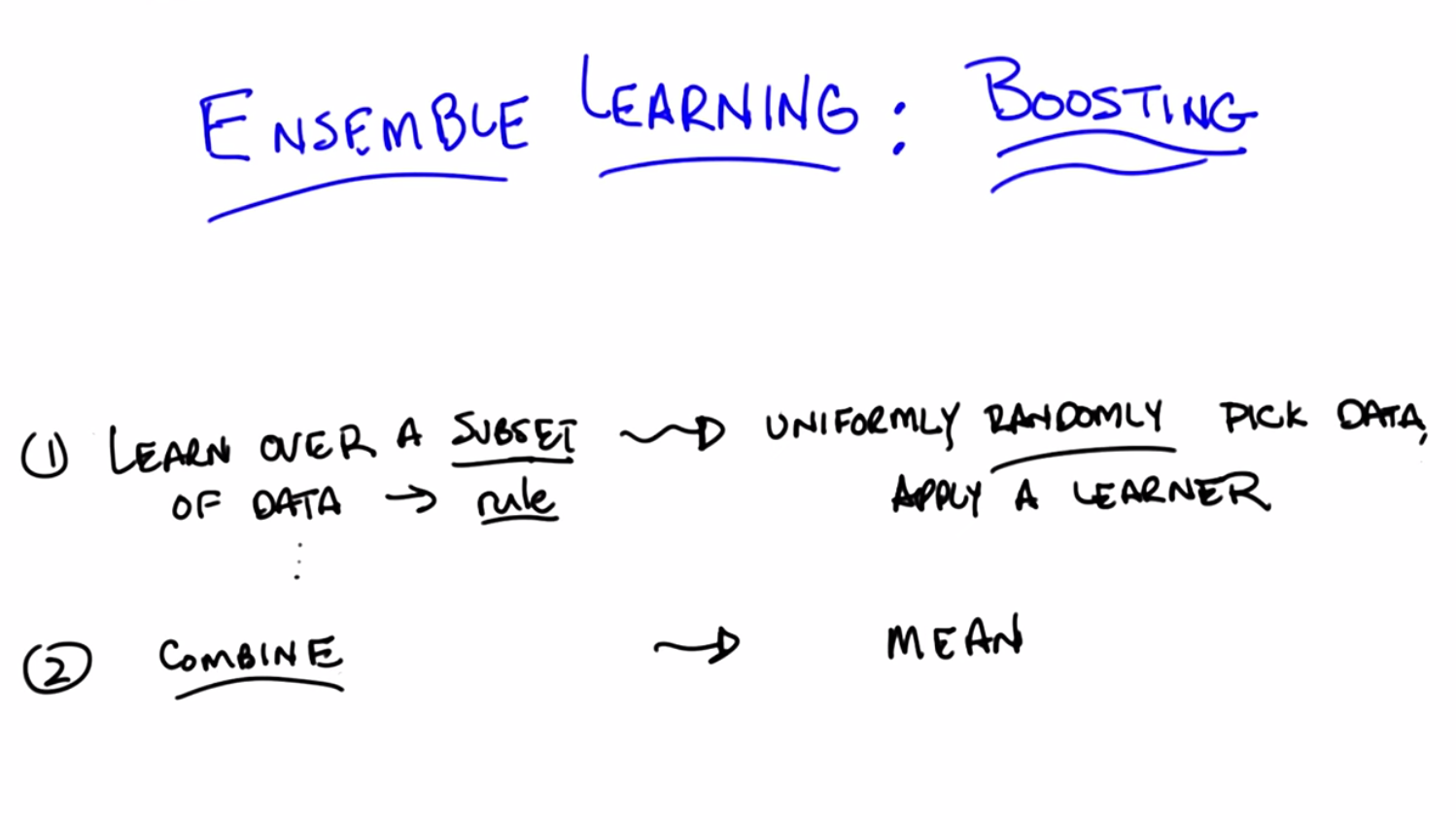
C: So, the characteristic of ensemble learning is first, that you take a bunch of simple rules, all of which kind of make sense and that you can see as sort of helping, but on their own, individually, don’t give you a good answer. And then you magically combine them in some way to create a more complex rule, that in fact, works really well. And ensemble learning algorithms have a sort of basic form to them that can be described in just one or two lines. So let me do that and then we can start wondering a little bit how we’re going to make that real. So here’s the basic form of an ensemble learning algorithm. Basically you learn over a subset of the data, and that generates some kind of a rule. And then you learn over another subset of the data and that generates a different rule. And then you learn over another subset of the data and that generates yet a third rule, and yet a fourth rule, and yet a fifth rule, and so on and so forth. And then eventually you take all of those rules and you combine them into one of these complex rules. So, we might imagine in the email case that I might look at a small subset of email that I know is already spam and discover that the word manly shows up in all of them and therefore pick that up as a rule. That’s going to be good at that subset of mail, but not necessarily be good at the other subset of mail. And I can do the same thing and discover that a lot of the spam mails are in fact short or a lot of them are just images or just URLs and so on and so forth. And that’s how I learn these rules – by looking at different subsets. Which is why you end up with rules that are very good at a small subset of the data, but aren’t necessarily good at a large subset of the data. And then after you’ve collected these rules, you combine them in some way, and there you go. And that’s really the beginning and the end of ensemble learning.
M: So wait. So, when you say manly was in a lot of the positive examples, do you mean like it distinguishes the positive and the negative examples? So it should also not be in the negative examples.
C: That’s right. That’s exactly right. So think of this as any other classification learning problem that you would have where you’re trying to come up with some way to distinguish between the positives and the negatives.
M: And why are we are looking at subsets of the data? I don’t understand why we can’t just look at all of the data.
C: Well, if we look at all of the data, then it’s going to be hard to come up with these simple rules. That’s the basic answer. Actually, ask me that question a little bit later, when we talk about overfitting, and I think I’ll have a good answer for you. Okay, so here we go Michael. This is Ensemble Learning. You learn over a subset of the data over and over again, picking up new rules, and then you combine them and you’re done.
Ensemble Learning Algorithm
scribble
slides
transcript
C: Here’s the Ensemble Learning algorithm. We’re done, Michael, we’re done with the entire lesson. We don’t have to do anything else anymore. We know that we’re supposed to look over subset of data, pick up rules, and then combine them. So, what else do you need to know in order to write your first Ensemble Learning algorithm?
M: So, I’m already kind of uncomfortable with this notion of “combine,” right? So, like, I can think of lots of really dumb ways to combine things. Like, choose one at random or, you know, I don’t know, add em all up and divide by pi. So, presumably, there’s got to be some intelligence in how this combination is taking place.
C: Yes, you would think so, but you’re not at all bothered about how you pick a subset?
M: Oh, I was imagining you meant random subsets.
C: Oh, so you already made an assumption about how we were going to pick a subset. You just weren’t sure how to combine them. Well actually, let’s explore that for a minute. Here’s kind of the dumbest thing you can imagine doing, and it turns out to work out pretty well. We’re going to pick subsets, by, I’m going to say uniformly, just to be specific about it. So we’re going to do the dumbest thing that we can think of, or rather, one of the dumbest things that we can think of. Or maybe we should say simplest (and not dumbest so as not to make a value judgment) thing that you can think of doing, which would be to just uniformly randomly choose among some of the data, and say that’s the data I’m going to look at, and then apply some learning algorithm to it. Is that what you were thinking of Michael?
M: Yeah.
C: Okay, so just: pick a subset of the data, apply a learner to it, get some hypothesis out, and get some rule out, and now I’m going to combine them. So since we’re being simple, why don’t we try doing something simple for combining? Let’s imagine, Michael, that we’re doing a regression. What’s the simplest thing you could do if you have ten different rules which tell you how you should be predicting some new data point? What’s the simplest thing you could imagine doing with them?
M: So, okay, so each of them spits out a number. I guess if we kind of equally believe in each of them, a reasonable thing to do would be to average.
C: Great. So, a very simple way of combining, in the case of regression, would be to average them. We’ll simply take the mean. And, by the way, why wouldn’t we equally believe in each of them? Each one of them learned over a random subset of the data. You have no reason to believe that one’s better than the other.
M: There’s a couple of reasons. One is that it could be a bad random subset. I don’t know how I would measure that.
C: It could be a good random subset.
M: Yeah. Then we’d want that to count more in the mean. I guess what I was thinking more in terms of maybe for some of the subsets, you know, it gets more error than others, or it uses a more complex rule than others or something.
C: I could imagine that. Actually, maybe we can explore how this sort of idea might go wrong. Let’s do that! Maybe we can do that with a quiz. You like quizzes, right?
M: They’re important.
Quiz: Ensemble Learning Outputs
scribble
slides

transcript
C: Okay, so here’s the quiz for you Michael, here’s the setup, you ready? You’ve got N data points. The learner that you’re going to use over your subsets is a 0th-order polynomial. The way you’re going to combine the output of the learners is by averaging them. So, it’s just what we’ve been talking about so far, and your subsets are going to be constructed in the following way. You uniformly randomly picked them and you ended up with N disjoint subsets, and each one has a single point in it that happens to be one of the data points.
M: Okay, I think I get that.
C: Right, so if you look over here on your left, you’ve got a graph of some data points and this is one subset, this is another subset, that’s another subset, that’s another subset, that’s another subset, that’s another subset, that’s another subset. Got it?
M: Yeah, now what do you want to know about it?
C: Now what I want to know is when you do your ensemble learning, you learn all these different rules and then you combine them. What is the output going to be? What does the ensemble output?
M: And you want a number?
C: I want a description and if the answer’s a number, that’s a perfectly fine description. But I’ll give you a hint, it’s a short description.
M: A short description of the answer. Okay, I’ll think about it.
C: Alright.
Answer
C: Okay Michael, have you thought about it? Do you know what the answer is?
M: Yeah. I think, you know, you asked it in a funny way, but I think, what you’re asking maybe was pretty simple. So let me see if I can talk it through. So, we’ve got N data points and each learner is a 0th-order polynomial. So you said the ensemble rule is that you learn over a subset. Well, we said that the thing that minimizes the expected error (or the squared error) of a 0thorder polynomial is just the average. So, if the sets are indistinct sets with one data point each, then each of the individual learners is just going to learn the average. The actual output value of each individual point is the average, and then the combining algorithm, to combine all the pieces of the ensemble into one answer, combines with the mean. So, it’s going to combine the mean of those, each of which is the data point, so it’s the mean of the data points. So, the ensemble outputs, I don’t know, I’d say average or mean?
C: Yes.
M: Or 0th-order polynomial of the data set, or, you know, a one node decision tree, or, uh…
C: A constant. Which happens to be the mean of the data. Haven’t we seen this before?
M: It seems to come up a lot when we are outputting very simple hypotheses.
C: Right. And the last time we did this, if I recall correctly, this is what happens if you do an unweighted average with k-NN where k equals n.
M: Oh, right. Like, like, right. n-NN.
C: n-NN.
M: Mm.
C: Mm, so we should probably do something a little smarter than this then. And, I thought that we might look at some of the housing data, because, no one’s started looking at the housing data yet. [LAUGH] Okay, so let’s look at that quickly and see if we can figure out how this works. And then see if we can do something a little bit better, even better than that. Okay?
Ensemble Learning An Example
scribble
slides

transcript
C: Alright, Michael, so, here’s what you have before you. You have the same housing data that we’ve looked at a couple of times before. For the sake of readability, I’ve drawn over some of the data points so that they’re easier to see, but this is exactly the data that we’ve always had. Okay?
M: Okay.
C: Now, you’ll notice that I marked one of them as green, because here’s what we’re going to do. I’m going to take the housing data you’ve got, I’m going to do some ensemble learning on it. And I’m going to hold out the green data point. Okay? So of the nine data points, you’re only going to learn on 8 of them. And I’m going to add that green data point as my test example and see how it does. Okay?
M: Okay. So that sounds like cross-validation.
C: It does. This is a cross-validation. Or you could just say, I just put my training set and my test set on the same slide.
M: Okay.
C: Okay, Michael, so the first thing I’m going to do is pick a random subset of these points. And just for the sake of the example, I’m going to pick five points randomly and I’m going to do that five times, so I’m going to have five subsets of five examples. And, by the way, I’m going to choose these randomly, and I’m going to choose them with replacement, so we’re not going to end up in the situation we ended up in just a couple of minutes ago where we never got to see the same data point twice. Okay?
M: Yeah.
C: Alright. So five subsets of five examples, and then I’m going to learn a 3rd-order polynomial. And I’m going to take those 3rd-order polynomials, I’m just going to learn on that subset, and I’m going to combine them by averaging. Want to see what we get? M: Oh, yeah, sure.
C: So here’s what you get, Michael. Here I’m showing you a plot over those same points, with the five different 3rd-order polynomials. Can you see them? M: Yeah. There’s like a bunch of wispy hairs.
C: Just like most 3rd-order polynomials. And as you can see they’re kind of similar. But some of them sort of veer off a little bit because they’re looking at different data points. One of them is actually very hard to see. It veers off because just, purely randomly, it never got to see the two final points.
M: I see. But they all seem to be pretty much in agreement between points three and four. There’s a lot of consistency there.
C: Right. Because just picking five of the subsets, you seem to be able to either get things on the end, or you get things in the middle and maybe one or two things on the end and it sort of works out. Even the one that doesn’t see the last two points still got to see a bunch of first ones and gets that part of the space fairly right.
M: Cool.
C: Okay. So the question now becomes: how good is the average of these compared to something we might have learned over the entire data set? And here’s what we get when do that. So what you’re looking at now Michael, is the red line: the average of all of five of those 3rd-order polynomials. And the blue line is the 4th-order polynomial that we learned when we did this with simple regression, a couple of lessons back.
M: Okay.
C: And you actually see they’re pretty close.
M: Why is one of them a 4th-order, and one a 3rd-order?
C: Well what I wanted to do is try a simpler set of hypotheses than we were doing when we were doing full blown regression. So 3rd-order’s simpler than 4th-order. So, I thought we’d combine a bunch of simpler rules than the one we used before and see how well it does.
M: You want to know how well it does?
C: I would!
M: Well it turns out that on this data set (and I did this many, many, many times just to see what would happen with many different random subsets), it typically is the case that the blue line always does better on the training set (the red points) than the red line does. But the red line almost always does better on the green point on the test set or the validation set.
C: Interesting.
M: That is kind of interesting. So wait, so let me get this straight. It seems sort of magical. So, so it learns an average of 3rd-degree polynomials, 3rd-order polynomials, which is itself a third order polynomial. But you’re saying it does better by doing this kind of trick than just learning a 3rd-order polynomial directly.
C: Yeah. Why might you think that might be? I have a guess, you tell me what you think.
M: Wow, so well, I mean, you know, the danger is often overfitting, overfitting is like the scary possibility. And so maybe kind of mixing the data up in this way and focusing on different subsets of it, I don’t know, it somehow manages to find the important structure as opposed to getting misled by any of the individual data points.
C: Yeah. That’s the basic idea. It’s kind of the same thing, at least that’s what I think. I think that’s a good answer. It’s basically the same kind of argument you make for cross-validation. You take a random bunch of subsets. You don’t get trapped by one or two points that happen to be wrong because they happen to be wrong because of noise or whatever and you sort of average out all of the variances and the differences. And oftentimes it works. And, in practice, this particular technique, ensemble learning, does quite well in getting rid of overfitting.
M: And what is this called?
C: So, this particular version, where you take a random subset and you combine by the mean, it’s called bagging.
M: And I guess the bags are the random subsets?
kC: Sure.
M: [LAUGH] That’s how I’m going to think of it.
C: That’s how I’m going to think of it. It also has another name which is called bootstrap aggregation. So I guess the different subsets are the boots.
M: [LAUGH] No, no, no, no – bootstrap usually refers to pulling yourself up by your bootstraps.
C: Yeah, I like my answer better. So, each of the subsets are the boots and the averaging is the strap. And there you go. So, regardless of whether you call it bootstrap aggregation or you call it bagging, you’ll notice it’s not what I said we were going to talk about during today’s discussion. I said we were going to talk about boosting. So we’re talking about bagging but we’re going to talk about boosting. The reason I wanted to talk about bagging is because it’s really the simplest thing you can think of and it actually works remarkably well. But there are a couple of things that are wrong with it, or a couple of things you might imagine you might do better that might address some of the issues and we’re going to see all of those when we talk about boosting right now.
Ensemble Boosting
scribble
slides

transcript
C: Okay so, let’s go back and look at our two questions we were trying to answer. And so far we’ve answered the first one – learn over a subset of data and define a rule – by choosing that subset uniformly randomly and applying some learning algorithm. And we answered the second question – how do you combine all of those rules of thumbs – by saying, you simply average them. And that gave us bagging. So Michael, I’m going to suggest an alternative to at least the first question and leave open the second one for a moment. That’s going to get us to what we’re supposed to be talking about today, which is boosting. So let me throw and idea at you and you tell me if you think it’s a good one. So rather than choosing uniformly randomly over the data, we should try to take advantage of what we are learning as we go along, and instead of focusing just kind of randomly, we should pick the examples that we are not good at. So what do I mean by that? What I mean by that is, we should pick a subset based upon whether the examples in that subset are hard. So what do you think of that?
M: Well, I guess it depends on how we think about hard, right? So it could be that it’s hard because it’s hard in some absolute sense, right, or it could be that it’s hard relative to, you know, if we were to stop now, how well we do?
C: Yeah, and I mean the latter.
M: Oh. Okay. Alright. Well I feel like that makes a lot of sense. I mean, certainly when I’m trying to learn a new skill, I’ll spend most of my energy on the stuff that I’m kind of on the edge of being able to do, not the stuff that I’ve already mastered. It can be a little dispiriting but I think I make faster progress that way.
C: Right, and if you go back to the example that we started out with, with spam, right? If you come up with a rule and you see it does a very good job on some of the mail examples but doesn’t do a good job on the other ones, why would you spend your time trying to come up with more rules that do well on the email messages you already know how to classify? You should be focusing on the ones you don’t know how to classify. And that’s the basic idea here between, the basic idea here behind boosting and finding the hardest examples.
M: Cool.
C: Okay. So that answers the first question. We’re going to look at the hardest examples and I’m going to define for you exactly what that means. I’m going to have to introduce at least one technical definition, but I want to make certain you have that. And the second one, the combining, well that’s a difficult and sort of complicated thing, but at a high level, I can explain it pretty easily by saying we are going to still stick with the mean.
M: Okay.
C: We’re voting, except this time, we are going to do a weighted mean. Now why do we want to do weighted mean? Well, I have to tell you exactly how we are going to weight it, but the basic idea is to avoid the sort of situations that we came across when we looked at the data before, where taking an average over a bunch of points that are spread out just gives you an average or a constant that doesn’t give you a lot of information about the space. So we’re going to weight it by something, and it’s going to turn out the way we choose to weight it will be very important. But just keep in your head for now that we’re going to try to do some kind of weighted average, some kind of weighted voting. Okay?
M: Sure. One of the things that’s scaring me at the moment though is this fear that by focusing on the hardest questions, and then, and then sort of mastering those, what’s to keep the learner from starting to kind of lose track of the ones it has already mastered? Like how, why does it not thrash back and forth?
C: So that’s going to be the trick behind the particular way that we do weighting.
M: Okay
C: So I will show you that in a moment, and it’s going to require two slightly technical definitions that we have been kind of skirting around this entire conversation. Okay?
M: Sure.
Ensemble Boosting Quiz
scribble
slides

transcript
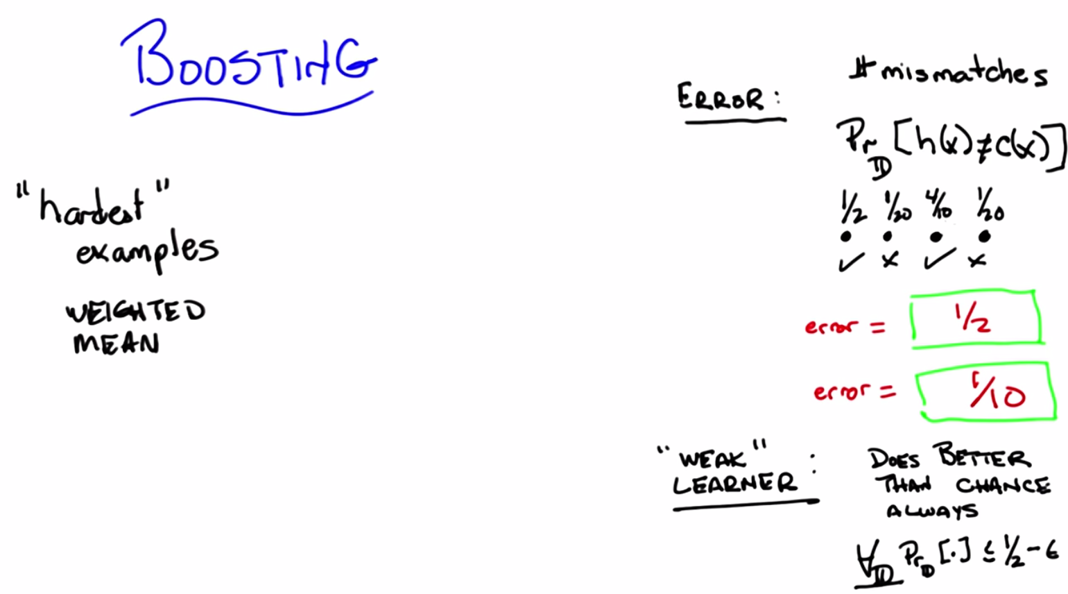
C: Alright so, the whole goal of what we’re going to add for boosting here is we’re going to expand on this notion of hardest examples and weighted mean. But before I can do that, I’m going to have to define a couple of terms. Okay. And you let me know, Michael, if these terms make sense. So, here’s the first one. The first one is error. So how have we been defining error so far?
M: Usually we take the squared difference between the correct labels and what’s produced by our classifier or regression algorithm.
C: That’s true. That is how we’ve been using error when we’re thinking about regression error. How about a notion of accuracy? About how good we are at, say, classifying examples? So let’s stick with classification for a moment.
M: Well, that would be the same as squared error, except that it’s doesn’t really need to be squared. That is to say, if the outputs are zeroes and ones, the squared error is just whether or not there’s a mismatch. So it could just be the total number of wrong answers.
C: Right. So, what we’ve been doing so far is counting mismatches. I like that word, mismatches. And we might define an error rate or an error percentage as the total number of mismatches over the total number of examples. And that tells us whether we’re at 85% or 92% or whatever, right? So that’s what we’ve been doing so far. But implicit in that, Michael, is the idea that every single example is equally important. So, that’s not always the case. Now you might remember from the very first talk that we had, we talked about distributions over examples. We said that, you know, learning only happens if your training set has the same distribution as your future testing set. And if it doesn’t, then all bets are off and it’s very difficult to talk about induction or learning. That notion of distribution is implicit in everything that we’ve been doing so far, and we haven’t really been taking it into account when we’ve been talking about error. So here’s another definition of error and you tell me if you think it makes sense, given what we just said. So, this is my definition of error. So the subscript D stands for distribution. So we don’t know how new examples are being drawn, but however they’re being drawn, they’re being drawn from some distribution, and I’m just going to call that distribution “D”, okay?
M: Mhm.
C: Right. So H is our old friend, the hypothesis. That’s the specific hypothesis that our learner has output. That’s what we think is the true concept, and C is whatever the true underlying concept is. So I’m going to define error as the probability, given the underlying distribution, that I will disagree with the true concept on some particular instance X. Does that make sense for you?
M: Yeah, but I’m not seeing why that’s different from number of mismatches in the sense that if we count mismatches on a sample drawn from D, which is how we would get our testing set anyway, then I would think that would be, you know, if it’s large enough, a pretty good approximation of this value.
C: So here Michael, let me give you a specific example. I’m going to draw four possible values of X. And when I say I’m going to draw four possible values of X, I mean I’m just going to put four dots on the the screen.
M: Hm.
C: Okay? And then I’m going to tell you that this particular learner output a hypothesis. Output you know, a potential function, that ends up getting the first one and the third one right, but gets the second and the fourth one wrong. So what’s the error here?
M: Mm.
C: So let’s just make sure that, that everybody’s with us. Let’s do this as a quiz.
M: Okay, so let’s ask the students what they think. So here’s the question again. You’ve output some hypothesis over the four possible values of x, and it turns out that you get the first and the third one right, and you get the second and the fourth one wrong. If I look at it like this, what’s the error rate?
Answer
C: Okay, Michael, what’s your answer?
M: It looks like, half of them are right and half of them are wrong. So, the number of mismatches, is, 2 out of 4 or a half.
C: Right, that is exactly the right answer because you got half of them right and half of them wrong. But it assumes that you’re likely to see all four of the examples equally often. So, what if I told you that that’s not in fact the case. So, here’s another example of error for you. What if I told you that each of the points is likely to be seen in different proportions. So you’re going to see the first one half the time. You’re going to see the second one 1/20th of the time. You’re also going to see the fourth one 1/ 20th of the time and the third one, 4/10ths of the time. Alright, so you got it Michael? One half, 1/ 20th, 4/10ths, and 1/20th.
M: Got it.
Quiz Ensemble Boosting Two
scribble
- You are counting the error.
slides
transcript
C: Okay. So, now I have a different question for you. Actually, I have the same question for you, which is, what is the error rate now? Go.
Answer
C: Okay, Michael, what’s the answer?
M: Well, it’s still a half. But I guess we really should take into consideration those probabilities. So the number of mismatches is half, but the actual number of errors, the expected number of errors is like well, 1/20th plus 1/20th, so like 1/10th. So it’s 90% correct, 10% error.
C: Right. That’s exactly right, so, what’s important to see here is that even though you may get many examples wrong, in some sense some examples are more important than others because some are very rare. And if you think of error, or the sort of mistakes that you’re making, not as the number of distinct mistakes you can make, but rather the amount of time you will be wrong, or the amount of time you’ll make a mistake, then you can begin to see that it’s important to think about the underlying distribution of examples that you see. You buy that?
M: Yeah.
C: Okay, so, that notion of error turns out to be very important for boosting because, in the end, boosting is going to use this trick of distributions in order to define what hardest is. Since we are going to have learning algorithms that do a pretty good job of learning on a bunch of examples, we’re going to pass along to them a distribution over the examples, which is another way of saying, which examples are important to learn versus which examples are not as important to learn. And that’s where the hardest notion is going to come in. So, every time we see a bunch of examples, we’re going to try to make the harder ones more important to get right than the ones that we already know how to solve. And I’ll describe in a minute exactly how that’s done.
M: But isn’t it the case that this distribution doesn’t really matter? You should just get them all right.
C: Sure. But now it’s a question of how you’re going to get them all right, which brings me to my second definition I want to make. And that second definition is a weak learner. So there’s this idea of a learning algorithm, which is what we mean by a learner here, being weak. And that definition is actually fairly straightforward – so straightforward, in fact, that you can sort of forget that it’s really important. And all a weak learner is, is a learner that, no matter what the distribution is over your data, will do better than chance when it tries to learn labels on that data. So what does better than chance actually mean? Well what it means is that, no matter what the distribution over the data is, you’re always going to have an error rate that’s less than 1/2. So what that means, sort of as a formalism, is written down here below: that for all D, that is to say no matter what the distribution is, your learning algorithm will have an expected error (the probability that it will disagree with the true actual concept if you draw a single sample) that is less than or equal to (epsilon). Now epsilon is a term that you end up seeing a lot in mathematical proofs, particularly ones involving machine learning. Epsilon just means a really, really small number somewhere between a little bigger than 0 and certainly much smaller than 1. So, here what this means technically is that you’re bounded away from 1/2. Another way of thinking about that is you always get some information from the learner. The learner’s always able to learn something. Chance would be the case where your probability is 1/2 and you actually learn nothing at all which kind of ties us back into the notion of information gain way back when with decision trees. So does that all make sense Michael?
M: I’m not sure that I get this right. Maybe we can do a quiz and just kind of nail down some of the questions that I’ve got.
C: Okay, sure. You got an idea for a quiz?
M: Sure.
Quiz Weak Learning
scribble
- Requirement for having a weak learner is fairly strong and an important condition.
slides
transcript
C: Okay Michael, so let’s make certain that you really grasp this concept of weak learning.
M: Mm-hm.
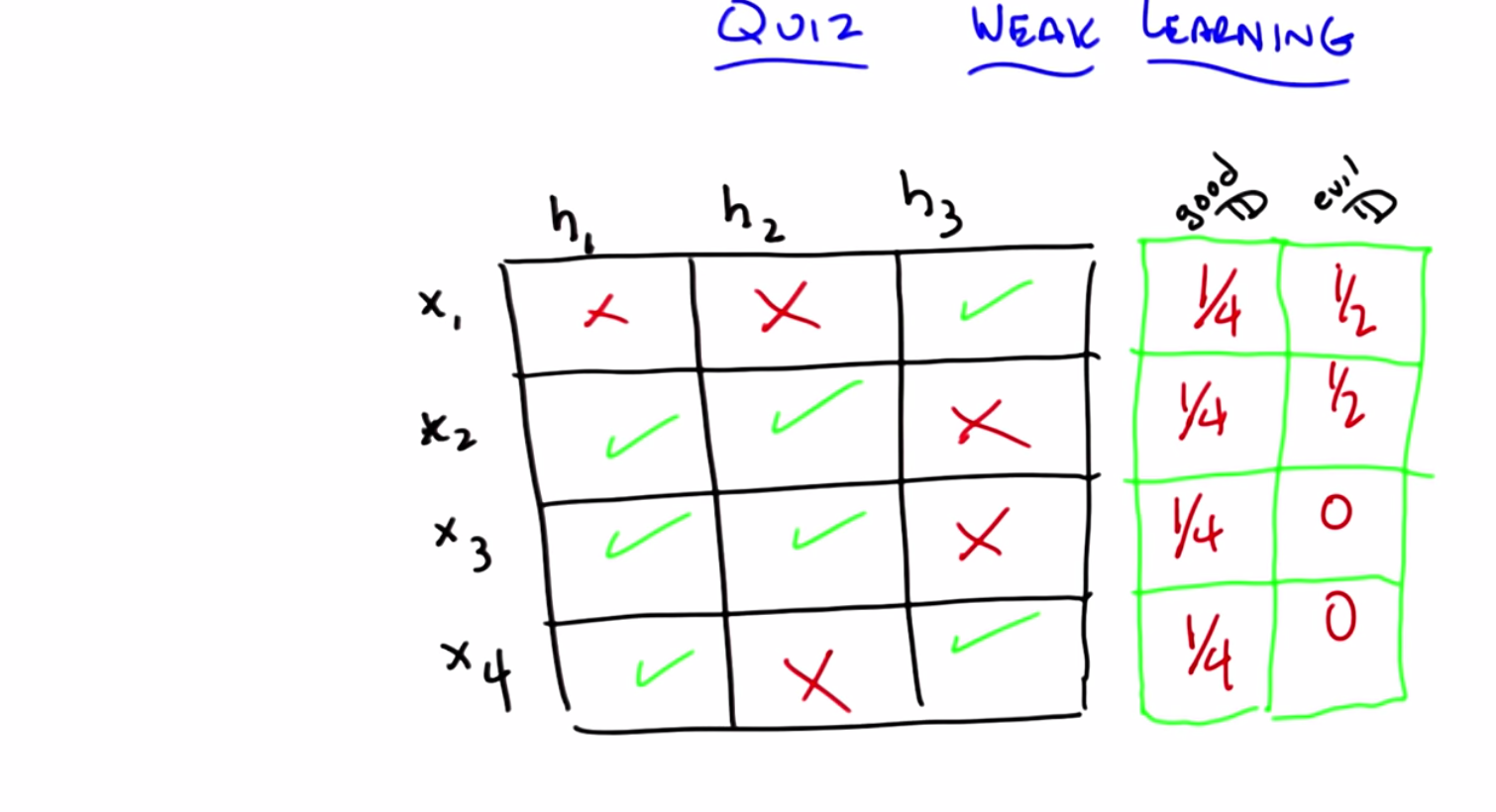
C: So, here’s a little quiz that I put together to test your knowledge. So, here’s the deal. I’ve got a little matrix here, it’s a little table, and across the top are three different hypotheses: hypothesis one, hypothesis two, and hypothesis three. So your entire hypothesis space consists only of these three hypotheses. Got it?
M: Got it.
C: Okay, your entire instance space consists entirely of only four examples; X1, X2, X3, and X4. Got it?
M: Got it.
C: I have an X in a square if that particular hypothesis does not get the correct label for that particular instance and I have a green check mark if that particular hypothesis does in fact get the right label for that example. So, in this case, hypothesis one gets examples 2, 3, and 4 correct but gets example one wrong, while hypothesis three gets one and four correct, but two and three incorrect.
M: I see. So, there’s no hypothesis that gets everything right.
C: Right.
M: So does that mean that we don’t have a weak learner, because then there’s some distributions for which any given hypothesis is going to get things wrong.
C: Maybe. Maybe not. Let’s see. Here’s what I want you to do. I want you to come up with the distribution over the 4 different examples, such that a learning algorithm that has to choose between one of those hypotheses will in fact be able to find one that does better than chance (by having an expected error greater than 1/2).
M: Okay.
C: Then if you can do that, I want you to see if you can find a distribution which might not exist, such that if you have that distribution over the four examples, a learning algorithm that only looked at H1, H2 and H3 would not be able to return one of them that has an expected error greater than 1/2.
M: So greater than 1/2 in this case would mean three out of four, correct? Oh no, no. Oh, you’re using, you want to use that definition that actually took into consideration the distribution.
C: Exactly. That’s the whole point. You always need to have some distribution over your examples to really know what your expected error is. M: Alright. And if there is no such evil distribution, should I just fill in zeros in all those boxes?
C: Yes, all zeros means no such distribution. You can do it in either case.
M: So if you put in all zeros you’re saying no such distribution exists. But otherwise it should add up to one down each of the columns.
C: It had better add up to one.
Answer
C: Okay Michael, you got answers for me?
M: Yeah, I think so. I decided that instead of solving this problem by thinking, I would just try a couple examples and see if I found things in both boxes. So, if I put equal weight on X1, X2, X3, and X4…
C: Mm-hm.
M: Then H1 gets three out of four correct, that’s 3/4. That’s better than 1/2.
C: Well done.
M: Then I fill that in the good boxes, quarters all the way down.
C: That’s a turtle, because it’s turtles all the way down [LAUGH].
M: No, no, it’s not though, it should be quarters all the way down. I thought you’d maybe draw a quarter.
C: I can’t draw a quarter, also I can’t draw a turtle obviously but still.
M: [LAUGH] Agreed. Alright, good.
C: Do you think anyone listening to this is old enough to get turtles all the way down?
M: Yeah, that’s a great joke. Everybody knows that joke.
C: And if people don’t know the joke, then we should pause this thing right now, and you should go look up turtles all the way down. And then come back. Okay.
M: It’s a really great joke if you’re computer scientist.
C: Yes, and if you don’t think it’s a good joke then you should probably be in a different field. Okay.
M: [LAUGH]
C: What about the evil distribution?
M: Okay, well, the issue here is that, because we spread all the probability out in the first hypothesis really well, so I said okay, well, let me put all the weight on the first example, X1.
C: Okay. So what did that look like?
M: H1 does very badly. It gets 100% error. H2 is 100% error. But H3 is 0% error.
C: yes.
M: So putting all the weight on X1 is no good. And if you look X2, X3, and X4, they all have the property that there’s always a hypothesis that gets them right. So I started to think, well, maybe there isn’t an evil distribution. And then I kind of lucked into putting 1/2 on both the first and the second one because I figured that that ought to work, but then I realized that’s an evil distribution because if you choose H1, H2, or H3, they all have exactly 50% error on that distribution.
C: Very good. So 1/2, 1/2, 0, 0, is a correct answer.
M: Now I don’t know if there are others. You know, certainly putting all the weight on X2 and X3 is no good, because H2 and H1 both get those. Putting all the weight on X3 and X4 is no good, because H1 gets all of those correct. In fact we have to have some weight on X1, because otherwise H1 is the way to go.
C: Right. So, yeah, that’s interesting. What does that mean in this case?
M: What do you mean?
C: So what does this tell us about how we build a weak learner for this example?
M: So what it tells us is, since there is a distribution for which none of these hypotheses will be better than chance, there is no weak learner for this hypothesis space, on this instance set.
C: Interesting. Is there a way to change this example so it would have a weak learner?
M: Um, I’m sure there is.
C: Like if we change X2/H3 to a check instead of an X. So if we made that a green one – here, I’ll make it a green one by using the power of computers.
M: Woah, special effects!
C: Yes.
M: So now there’s no way to put weight on any two things and have it fail. I don’t know, my intuition now is that this should have a weak learner. Okay, well, how would we prove that?
C: I don’t know, but maybe we should end this quiz.
M: Yeah, I think we should end this quiz and leave it as an exercise to the listener. By the way, we should point a couple of things here though, Michael. One is that if we had more hypotheses and more examples and we had the X’s and the Y’s in the right places, then there’d be lots of ways to get weak learners for all the distributions because you’d have more choices to choose from. What made this one particularly hard is that you only had three hypotheses and not all of them were particularly good.
C: Sure, yeah. I mean, you can have many, many hypotheses. If they’re all pretty bad, then you’re not going to do very well.
M: Well, it would depend upon if they’re bad on very different things. But you’re right, if you have a whole lot of hypotheses that are bad at everything, you’re going to have a very hard time with a weak learner. And if you have a whole bunch of hypotheses that are good at almost everything, then it’s pretty easy to have a weak learner.
M: Okay, this is more subtle than I thought. So that’s, that’s interesting.
C: Right. So the lesson you should take away from this is: if you were to think about it for 2 seconds you might think that finding a weak learner is easy. Often, it is, but if you think about it for 4 seconds, you realize that’s actually a pretty strong condition. You’re going to have to have a lot of hypotheses that are going to have to do well on lots of different examples, or otherwise, you’re not always going to be able to find one that does well no matter what the distribution is. So it’s actually a fairly strong, and important condition.
Boosting In Code
scribble
slides

transcript
C: All right Michael, so here’s boosting in pseudocode. Okay, let me read it out to you, then you can tell me if it makes sense. So we’re given a training set. It’s made up of a bunch of xi , yi pairs.
You know, x is your input and y is your output. And for reasons that’ll be clear in a moment, all of your labels are either -1 or +1, where -1 means not in the class and +1 means you’re in the class. So this is a binary classification task. Does that make sense?
M: So far.
C: Okay. And then what you’re going to do is, you’re going to loop at every time step, let’s call it t, from the first time step 1, to some big time in the future – we’ll just call it T and not worry about where it comes from right now. The first thing you’re going to do is you’re going to construct a distribution. And I’ll tell you how in a minute, Michael, so don’t worry about it. And we’ll just call that Dt So, this is your distribution over your examples at some particular time t. Given that distribution, I want you to find a weak classifier. I want your weak learner to output some hypothesis. Let’s call that Ht , the hypothesis that gets produced at that time step, and that hypothesis should have some small error. Let’s call that error , because it’s a small number, such that it does well on the training set, given the particular distribution, which is to say, that the probability of it being wrong (disagreeing with the training label) is small with respect to the underlying distribution.
M: So just to be clear there, could be as big as slightly less than 1/2. Right? It doesn’t have to be tiny. It could actually be almost 1/2. But it can’t be bigger than 1/2.
C: That’s right, no matter what happens. It could even equal 1/2, but, you know, we can assume, although it doesn’t matter for the algorithm, that the learner is going to return the best one that it can with some error. But regardless, it’s going to satisfy the requirements of a weak learner and all I’ve done is copy this notion of error over to here. Ok?
M: Awesome!
C: Ok. So, you’re going to do that and you’ll do that for a whole bunch of time steps, constantly finding hypotheses at each time step Ht with small error , constantly making new distributions, and then eventually, you’re going to output some final hypothesis. I haven’t told you yet how you’re going to to get the final hypothesis, but that’s the high level bit. Look at your training data, construct distributions, find a weak classifier with low error, keep doing that you have a bunch of them, and then combine them somehow into some final hypothesis. And that’s high level of algorithm for boosting, okay?
M: Okay, but you’ve left out the two really important things, even apart from how you find a weak classifier, which is where do we get this distribution and where do we get this final hypothesis?
C: Right, so let me do that for you right now.
The Most Important parts
scribble
- What is zt?
slides

transcript
C: Okay Michael, you’ve called my bluff. You said I’ve left out the most important parts, and you are right. So, I’m going to tell you how to construct the most important parts. Let’s start with the distribution. So, let’s start with the base case, and that is the distribution at the beginning of time, D1. So this distribution is going to be over each of the examples and those examples are indexed over i. I’m simply going to set that distribution to be uniform. So, how many examples do we have, Michael? Let’s call it n.
M: Okay.
C: Why not, because we do that for everything else and I’m going to say that for every single example, they happen 1/n times, that is, a uniform distribution. Now, why do I do that? Because I have no reason to believe, for the purposes of this algorithm, that any given example is better than any other example, more important than any other example, harder than other example, or anything else. I know nothing. So, see if you can learn over all of the examples. Are you with me?
M: Yeah, cause I feel like if it actually solves that problem, we’re just done.
C: Yes, and that’s what you always want. But that’s the easy case. So I start out with a uniform distribution because that’s what you usually do when you don’t know anything. But what are you going to do while you’re in the middle? So, here’s what I am going to do, Michael. At every time step t, I’m going to construct a new distribution, Dt+1. Okay so, here’s how we’re going to construct the distribution at every time step. I’m going to create the new distribution Dt+1 to be the equation located to the right of the screen. So that’s pretty obvious right? So what do each of those terms mean? Let me just try to explain what each of the parts mean. So, we know that D is our distribution and it’s some number, where, over all the examples, it adds up to 1. And it’s a stand-in, we know, because I said this at the beginning, for how important a particular example is – how often we expect to see it. And that’s the trick that we’re using with distributions. So, I’m going to take the old distribution for a particular example and I’m going to either make it bigger or smaller, based upon how well the current hypothesis does on that particular example. So, there’s a cute little trick here. We know that Ht always returns a value of either -1 or +1 because that’s how we define our training set. So, Ht is going to return -1 or +1 for a particular xi yi , which is the label with respect to that example, is also always going to be +1 or -1. And is a constant which I will get into a little bit later. Just think of it right now as a number. So what happens, Michael, if the hypothesis at time t for a particular example xi agrees with the label that is associated with that xi?
M: Well, hang on, you say the alpha’s a number. Is it a positive number? A number between 0 and 1? A negative number? What kind of number? Does it not matter? I think it matters.
C: That’s a good question. It matters eventually. But right now, that number is always positive.
M: Positive, alright. So almost like a learning rate kind of thing, maybe.
C: It’s a learning rate kind of thing, sort of.
M: Alright, so, good. So, the yi times hi is going to be 1 if they agree, and -1 if they disagree.
C: Exactly, so if they both say +1, +1 times +1 is 1. If they both say -1, -1 times -1 is 1. So, it’s exactly what you say when they agree, that number is 1. And when they disagree, that number is -1. , which I define above, is always a positive number. So, that means when they agree, that whole product will be positive, which means you’ll be raising e to some negative number. When they disagree, that product will be negative, which means you’ll be raising e to some positive number. So, let’s imagine they agree. So you’re going to be raising e to some negative number. What’s going to happen to the relative weight of Dt(i)?
Quiz: When D agrees
scribble
- zt is defined as whatever normalization constant that you will need in order for it work out be a distribution.
slides
transcript
C: So, Michael wants us to do a quiz because Michael likes quizzes because he thinks you like quizzes, so, I want you to answer this question before Michael gets a chance to. What happens to Dt(i) when the hypothesis ht that was output by the example agrees with the particular label yi? Okay, so we have four possibilities when they agree. One is the probability of you seeing that particular example increases. That is, you increase the value of Dt(i), or the probability of you seeing that example decreases, or it stays the same when they agree or, well, it depends on exactly what’s going on with the old value of Dt(i) and and all these other things, so you can’t really give just one of those other three answers. Those are your possibilities. They’re radio buttons, so only one of them is right. Go.
Answer
C: Okay Michael, what’s the answer?
M: Alright, so you kind of were walking us through it, but basically if yi and ht agree, that means they’re both negative or they’re both positive, so when we multiply them together, we get 1. 1 times whatever our thing is, a positive number, is going to be positive. We’re negating that, so it’s negative. e to the negative power is something between zero and one, so that’s going to scale it down. So, it looks like it could depends on the normalization.
C: That’s a good point. The zt term is, in fact, whatever normalization constant you need at time t in order to make it all work out to be a distribution (sum to 1).
M: Correct. Then it’s not going to change.
C: True.
M: But if some of them are correct and some of them are incorrect, the ones that are correct are going to decrease. And the ones that are incorrect are going to increase.
C: That’s right, so what’s the answer to the quiz?
M: Depends.
C: That’s true, it does. That’s exactly the right answer. It depends on what else is going on, you’re correct.
M: But I feel like it should be decreases because that’s mainly what happens.
C: That’s also fair. The answer is, if this one is correct, that is they agree, and you disagree on at least one other example, it will, in fact, decrease. So I could ask a similar question, which is, well what happens when they disagree and at least one other example agrees. Then what happens?
M: Yeah, then that should increase.
C: Right.
M: Oh. It’s going to put more weight on the ones that it’s getting wrong.
C: Exactly. And the ones that it’s getting wrong must be the ones that are harder. Or at least that’s the underlying idea. All right, Michael, so you got it? So you understand what the equation’s for?
M: Yeah, it seemed really scary at first but it seems marginally less scary now because all it seems to be doing is putting more weight on those answers that it was getting wrong, and the ones that it’s getting right, it puts less weight on those and then you know, the loop goes around again and it tries to make a new classifier.
C: Right, and since the ones that it’s getting wrong are getting more and more weight, but we are guaranteed, or at least we’ve assumed, that we have a weak learner that will always do better than chance on any distribution, it means that you’ll always be able to output some learner that can get some of the ones that you were getting wrong, right.
Final Hypothesis
scribble
slides

transcript
C: So that ties together what constructing D does for you, and connects it to the hardest examples. So now, that gets us to a nice little trick where we can talk about how we actually output our final example. So, the way you construct your final example is basically by doing a weighted average based upon this . So the final hypothesis is just the sgn (sign) function of the weighted sum of all of the rules of thumb – all of the weak classifiers that you’ve been picking up over all of these time steps – where they’re weighted by the ’s. And remember, the is . That is to say, it’s a measure of how well you’re doing with respect to the underlying error. So, you get more weight if you do well than if you do less well, where you get less weight. So what does this look like to you? Well, it’s a weighted average based on how well you’re doing or how well each of the individual hypotheses are doing and then you pass it through a thresholding function where, if it’s below zero, you say negative and, if it’s above zero, you say positive and, if it’s zero, you just throw up your hands and and return zero. In other words, you return the sign of the number. So you are throwing away information there, and I’m not going to tell you what it is now, but when we go to the next lesson, it’s going to turn out that that little bit of information you throw away is actually pretty important. But that’s just a little bit of a teaser. Okay so, this is boosting, Michael. There’s really nothing else to it. You have a very simple algorithm which can be written down in a couple of lines. The hardest parts are constructing the distribution, which I show you how to do , and then simply bringing everything together, which I show you how to do.
M: Alright yeah, I think it doesn’t seem so bad and I feel like I could code this up, but I would be a little happier if I had a handle on why is the way that it is. C: Well there’s two answers. The first answer is: you use natural logs because you’re using exponential and that’s always a cute thing to do. And of course, you’re using the error term as a way of measuring how good the hypothesis is. And the second answer is, it’s in the reading you were supposed to have done. [LAUGH] So, go back and read the paper now that you’ve listened to this and you will have a much better understanding of what it’s trying to tell you.
M: Thanks.
C: You’re welcome. I’m about helping others, Michael, you know that.
Three Little Boxes
scribble
slides
transcript
C: So, Michael, I want to try to convince you other than the fact that it’s an algorithm with symbols that, it sort of works, at least informally. And then, I’m going to do what I always do and refer you to actually read the text to get the details. But before I do that, I wanted to go through an example if you think that would help.
M: I would like an example.
C: Okay. So, let’s go through an example. So, here’s a very simple example. So, I’ve got three little boxes on the screen. Can you see them?
M: Yeah.
C: Now, they’re the same boxes. I’ve drawn them up here beforehand because I’m going to solve this problem in only three steps.
M: Hey those boxes are really nice, did you get help from our trusty course developer?
C: I did in fact did get help from our trusty course developer. And when I say help, I mean he did this.
M: Oh, thanks Pushkar.
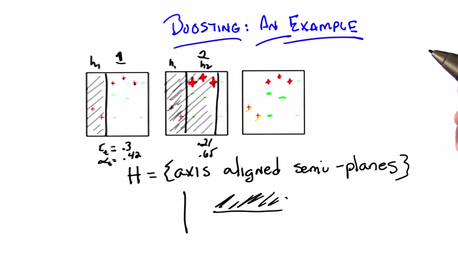
C: Yes, Pushkar is wonderful. Now what’s really cool about this is that Pushkar has already let you know that we’re going to be able to do this in 3 simple steps. And I’m going to be able to animate it, or at least hopefully it’ll look animated by the time we’re done with all the editing. So just pay attention to the first box for now. You have a bunch of data points; red plusses (+) and green minuses (-) with the appropriate labels and they all live in this part of the plane. By the way, what do you call a part of the plane? I know you have line segments, what’s like, a subpart of a plane?
M: Looks like a square to me.
C: Yes it is, but I mean, what do you call them? You don’t call it a plane segment, do you? What do you call it?
M: A region.
C: A square region, fine. So it’s a square region on a plane. And we want to figure out how to be able to correctly classify these examples. Okay, so that is nothing new there. We just want to be able to come up with something. So now we have to do what we did in the quiz, which is to specify what our hypothesis space is. So here’s our hypothesis space. So the hypothesis space is the set of axis-aligned semi-planes. You know what that means?
M: Mm, no.
C: Well for the purpose of this example it means, I’m going to draw a line, either horizontal or vertical, and say that everything on one side of that line is positive and everything on the other side of that line is negative.
M: I see. Okay, good.
C: Right. And their axes align because it’s only horizontal and vertical, and they’re semi-planes because the positive part of it is only in part of the plane. Okay, so I’m going to just walk through what boosting would end up doing with this particular example or what a boosting might do with this particular example given that you have a learner that always chooses between axis-aligned semi-planes. Okay?
M: Yeah.
C: So let’s imagine we ran our boosting algorithm. Now in the beginning, it’s step 1. All of the examples look the same because we have no particular reason to say any are more important than the other or any are easier or harder than the other. And that’s just the algorithm we had before. We run through and we ask our learner to return some hypothesis that does well in classifying the examples. It turns out that though there are many, and in fact, there are an infinite number of possible hypotheses you could return, one that works really well is one that looks like a vertical line that separates the first two data points from the rest.
M: That is what I was guessing.
C: Of course it was. And what I’m saying here is that everything to the left of this line is going to be positive and everything to the right is going to be negative. So if you look at this what does this hypothesis do? So it gets correct (correctly labeled positive) the two plusses to the left. Right?
M: Correct.
C: And it gets correct all of the minuses as well.
M: Correct.
C: Right? But it gets wrong the three plusses on the right side. So it gets, this wrong, this wrong, and this wrong.
M: Right, the Three Plusketeers.
C: Exactly. [LAUGH] The Three Plusketeers. That’s actually pretty good. So I’m just going to ask you to trust me here but it turns out that the specific error here is 0.3 and if you stick that into our little you end up, our little, our little formula for , you end up with equal to 4.2.
M: That’s not obvious to me, but…
C: See, it’s not always obvious. Okay. Good. So there you go and that’s just what happens when you stick this particular set in there. So now we’re going to construct the next distribution. Right? And what’s going to happen in the next distribution?
M: So the ones that it got right should get less weight and the ones that it got wrong should get more weight so those Three Plusketeers should become more prominent somehow.
C: That’s exactly what happens. They become, I’m just going to draw them as much thicker and bigger to kind of emphasise that they’re getting bigger, and it’s going to turn out that everything else is going to get smaller which is a lot harder to draw here. So I’m just going to kind of leave them their size, so they sort of get normalized away. Okay?
M: I have a guess as to what the next plane should be. I think that we should cut it underneath those plusses but above the green minuses. And that should get us three errors. The two plusses on the left and the minus on the top will be wrong but they have less weight than the three plusses we got right, so this going to be better than the previous one.
C: So, that’s possibly true. But it’s not what the learner output.
M: Oh!
C: Let me tell you what the learner did output though. This learner output by putting a line to the right of the three plusses, because he’s gotta get those right in saying that everything to the left is in fact, positive. So, does that seem like a reasonable one to you?
M: Well, it does better than half. I guess that’s really all what we’re trying to do, but it does seem to do worse than what I suggested.
C: Well, let’s see, it gets the three that you were really, really doing poorly on right, but then so did yours. And it picks up still the other two which it was getting right. And it gets wrong these three minuses which aren’t worth so much. So is that worse than what you suggested? No, it gets wrong, oh, the three minuses. Oh, it gets correct those two red plusses on the left. So it gets three things wrong. So that’s just as good as what I suggested. Okay, I agree.
M: Okay good. So the area of this step by the way, turns out to be 0.21 and the at this time step turns out to be 0.65. So that’s pretty interesting, so we got a bunch of these right and a bunch of these wrong. So what’s going to happen to the distribution over these examples?
C: The ones that got it wrong should get pushed up in weight and which ones are those? The green minuses in the middle patch.
M: Right.
C: They should become more prominent. The plusses, the three Plusketeers, should become less prominent than they were but it still might be more prominent than they were in the beginning. And maybe because in fact the , let’s see: the alpha is bigger, so, it will have actually a bigger effect on bringing it down. M: Yeah I guess so, but it, it’ll still be more prominent than the other ones that haven’t been bumped.
C: Yeah the ones that you’ve never gotten wrong.
M: Hm.
C: So they’re really going to disappear. These plusses are going to be a little bit bigger than the other plusses, but they’re going to be smaller than they were before. The three greens in the middle are going to be bigger than they were before. But those two plusses are going to be even smaller, and these two minuses are going to be smaller. So, what do you think the third hypothesis should be?
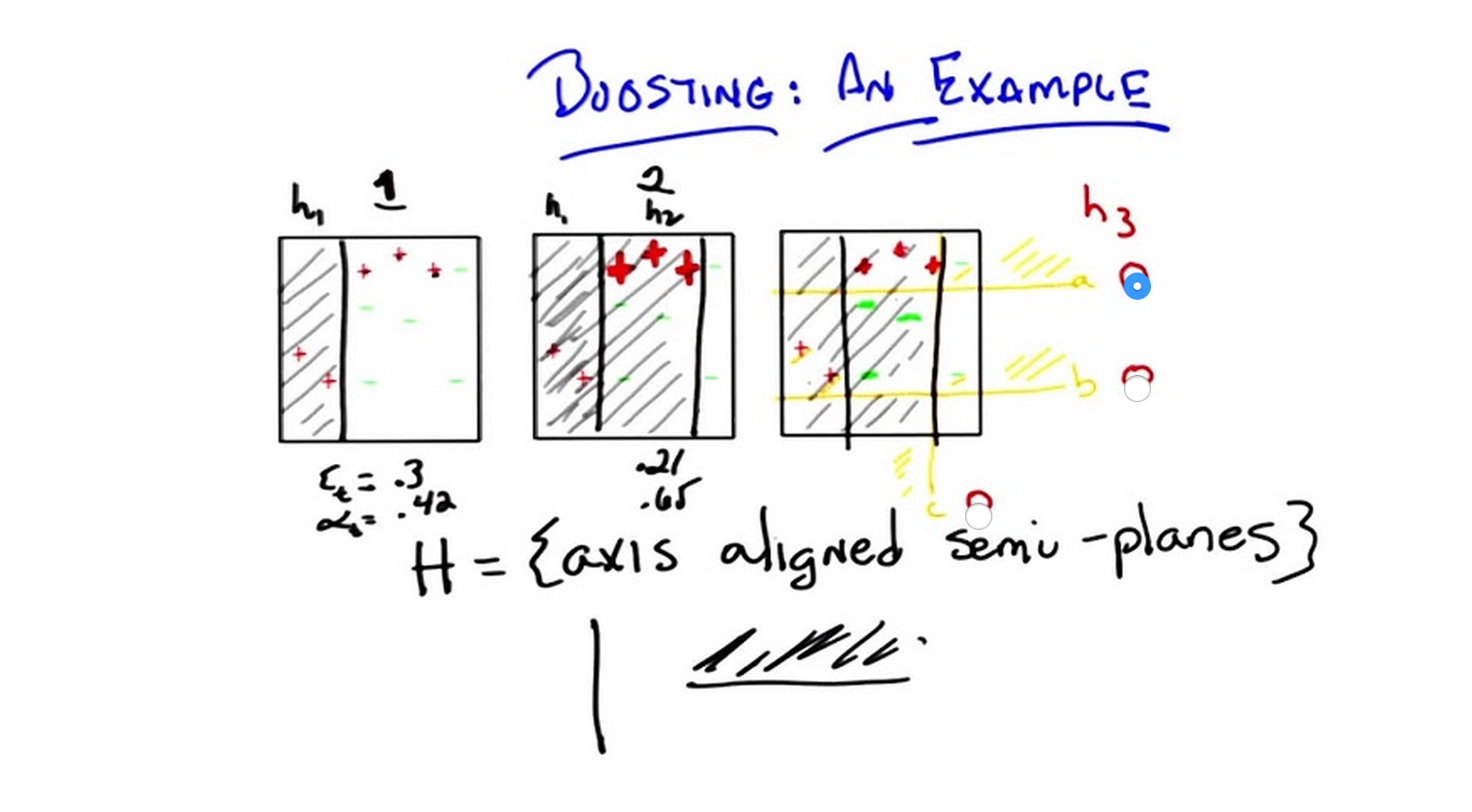
Which Hypothesis
scribble
slides
transcript
C: Okay, so Michael wanted to have a quiz here, because Michael again, likes those sort of things and, and I like to please Michael. So, we came up with three possibilities, one of which we hope is right. And I’ve labeled them here in orange: A, B, and C and put little radio boxes next to ‘em, so you could select ‘em. So which of those three hypotheses is s a good one to pick next? So, A is a horizontal line that says everything above it should be a plus. B is a another horizontal line that says everything above it should be a plus. And C is a vertical line, like the last two hypotheses that we found, that says everything to the left should be a plus. So, which do you think is the right one? Go.
Answer
C: Alright Michael, what’s the answer? M: So, of those others,
C is pretty good because it does separate the plusses from the minuses. We even liked it so much we used it in round two.
C: Mh-hm.
M: But it doesn’t look as good to me as A, because A actually does a good job of separating the more heavily weighted points. So I would say A.
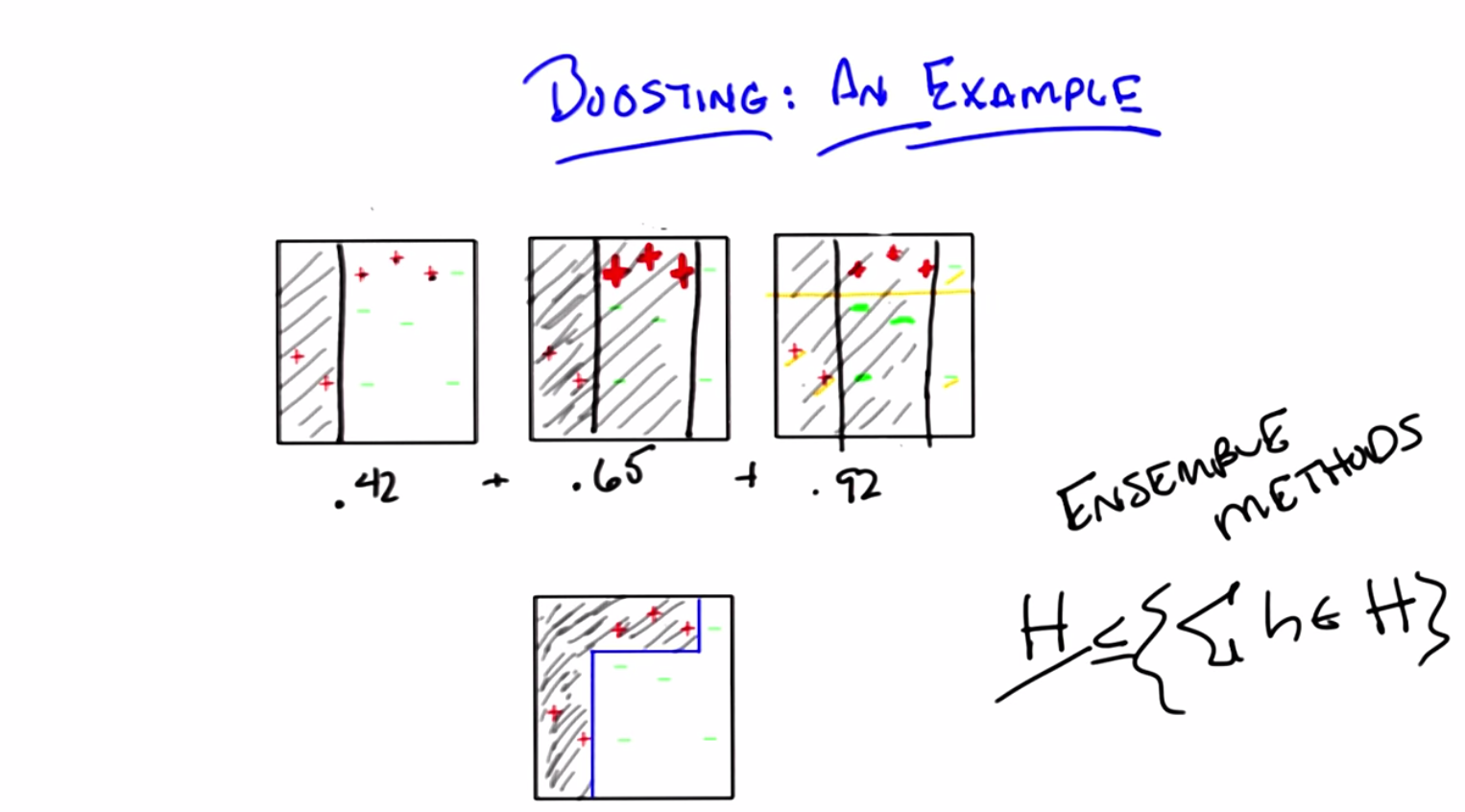
C: So, in fact, that is what our little learning system shows. It shows A. Now, through the trick of animation, I leave you with A. And that is exactly the right answer. By the way, Michael, if you look at these three hypotheses and their weights, you end up with something kind of interesting. If you look at this third hypothesis that’s chosen here, it turns out to have a very low error (that is decreasing) of 0.14, and it has a much higher of 0.92. Now if you look at these weights and you add them up, you end up with a cute little combination. So, let me draw that for you. If you take each of the three hypotheses that we produced and you weight them accordingly, you end up with the bottom figure.
M: No way.
C: Absolutely.
M: That’s kind of awesome. So what you’re saying is that, even though we were only using axisaligned semi planes for all the weak learners, at the end of the day, it actually kind of bent the line around and captured the positive and negative examples perfectly.
C: Right. Does that remind you of anything else we’ve talked about in the past?
M: Everything. Nothing. I mean, so with decision trees, you can make the shapes like that.
C: That’s true.
M: And the fact that we’re doing a weighted combination of things reminds me of neural nets.
C: Yeah. And it should remind you of one other thing.
M: I’m imagining that you want me to say nearest neighbors, but I can’t quite make the connection.
C: Well, you’ll recall in our discussion with nearest neighbors, when we did weighted nearest neighbor. In particular, we did weighted linear regression. We were able to take a simple hypothesis and add it together in order to get a more complicated hypothesis.
M: That’s true, because it’s local.
C: Right, exactly, because it’s local, and this is a general feature of ensemble methods. If you try to look at just some particular hypothesis class H, because you’re doing weighted averages over hypotheses drawn from that hypothesis class, this hypothesis class is at least as complicated as this hypothesis class and often is more complicated. So you’re able to be more expressive, even though you’re using simple hypotheses, because you’re combining them in some way.
M: I’m not surprised that you can combine simple things to get complicated things. But I am surprised that you can combine them just with sums and get complicated things because sums often act very, you know, sort of, friendly. It’s a linear combination, not a nonlinear combination.
C: Actually, Michael, part of the reason you get something nonlinear here is because you’re passing it through a nonlinearity at the end.
M: The sine.
C: Yeah, that’s a good thing, we should ponder that.
Good Answers
scribble
- You must pick up information all the time.
slides

transcript
C: Okay Michael, so we’ve done our little example. I want to ask you a quick question and try to talk something through with you and then we can start to wrap up. Okay.
M: Awesome.
C: Alright, so, here is my quick question. Now, in the reading, which I know you’ve read, there’s a proof that shows that boosting not only, you know, does pretty things with axis-aligned semi-planes, but also that it will converge to good answers and that it will find good combined hypotheses. You know, we could go look at the reading and write down a proof that shows that boosting does well and there’s one in the reading, or we could talk about an intuition. So, if a student were to find you somewhere and said, “I read the proof, I’m kind of getting it, but do you have a good sort of intuition about why boosting tends to do well?” What do you think you would tell them? Could you think of something simple? I’ve been struggling with this for a while.
M: No. [LAUGH].
C: Okay, well, then let me try something on you and you can tell me if it sort of makes sense. So this is just an intuition for why, for why boosting tends to do well. Okay, so what does boosting do? Okay. Boosting basically says, if I have some examples that I haven’t been able to classify well, I’m going to re-rate all my examples so that the ones I don’t do well on become increasingly important. Right, that’s what boosting does. Yes?
M: Yes.
C: Right, that’s what this whole, whole bit of D is all about. It’s all about re-weighting based on difficulty and hardest. And we know that we have the notion of a weak learner. That no matter what happens for whatever distribution, we’re always going to be able to find some hypothesis that does well. So, if I’m trying to understand why boosting in the end, why the final hypothesis that I get at the end, is going to do well, I can try to get a feeling for that by asking, well, under what circumstances would it not do well? So, if it doesn’t do well, then that means there has to be a bunch of examples that it’s getting wrong, right?
M: Mm hm.
C: That’s what it would mean not to do well, agreed?
M: Yeah.
C: Okay. So how many things could it not get right? How many things could it misclassify? How many things could it get incorrect? Well, I’m going to argue Michael, that that number has to be small. There cannot be a lot of examples that it gets wrong. So do you want to know why? Do you want to know my reasoning for why?
M: Yeah.
C: So, here’s my reasoning, let’s imagine I had a number of examples at the end of this whole process. I’ve done it T times. I’ve gone through this many times and I have some number of examples that I’m getting wrong. If I were getting those examples wrong, then I was getting them wrong in the last time step, right? And, since I have a distribution and I re-normalize, and it has to be the case that at least half of the time, I am correct, the number of things I’m getting wrong has to be getting smaller over time. Because let’s imagine that I was at a stage where I had a whole bunch of them wrong. Well, then I would naturally renormalize them with a distribution so that all of those things are important. But if they were all important, the ones that I was getting wrong, the next time I run a learner, I am going to have to get at least half of them right, more than half of them are right. Is that make sense? M: It does, but it, but what scares me is, okay, why can’t it just be the case that the previous ones which were getting right start to get more wrong as we shift our energy towards the errors.
C: Yeah, why is that?
M: I don’t know. But are we working up to some kind of you know, logarithmic kind of thing where after each time step you are knocking off half of them and therefore…
C: I don’t know. Do you remember the proof.
M: The proof.
C: I mean what goes on is that you get, sort of, this exponentially aggressive weighting over examples, right?
M: Yeah.
C: And you’re driving down the number of things you get wrong sort of exponentially quickly, over time. That’s why boosting works so well and works so fast.
M: I get that we’re, the we’re quickly ramping up the weights on the hard ones. I don’t get why that’s causing us to get fewer things wrong over time. So like, in your example that you worked through, that had the error in the alphas and the errors kept going down and the alphas kept going up.
C: Right.
M: Like, is that necessarily the case?
C: Well, what would be the circumstances under which it isn’t the case? How would you ever go back and forth between examples? Over time, every new hypothesis gets a vote based upon how well it does on the last, difficult let’s say, distribution. So even if the ones that you were getting right, you start to get wrong, if you get them increasingly wrong, that error’s going to go down and you’re going to get less of a vote. Because et is over the current distribution and it’s not over the sum of all the examples you’ve ever seen.
M: Understand.
C: So does that make sense? Is that right?
M: I don’t know. I don’t have the intuition, it seems like it could be, because we keep shifting the distribution, it could be that the error is going up. Like if the error could be low, why can’t we just make it low from the beginning?
C: Right.
M: Like, I feel like the error should be going up, because we’re asking it harder and harder questions as we go.
C: No, no, no, because we’re asking it harder and harder questions, but even though we’re asking it harder and harder questions, it’s forced to be able to do well on those hard questions. It’s forced to, because it’s a weak learner. That’s why having a weak learner is such a powerful thing.
M: But why couldn’t we like on, on iteration 17, have something where the weak learner works right at the edge of its abilities and it just comes back with something that’s 1/2 minus epsilon.
C: That’s fine. But it has to always be able to do that. If it’s 1/2 minus epsilon, the things it’s getting wrong will have to go back down again.
M: No, no I understand that. What I’m saying is that, why would the error go down each iteration?
C: Well, it doesn’t have to, but it shouldn’t be getting bigger.
M: Why shouldn’t it be getting bigger?
C: So, imagine the case that you’re getting. You are working at the edge of your abilities. You get half of them right roughly and half of them wrong. The ones you got wrong would become more important, so the next time around you’re going to get those right versus the other ones. So you could cycle back and forth I suppose, in the worst case, but then you’re just going to be sitting around, always having a little bit more information. So your error will not get worse, you’ll just have different ones that are able to do well on different parts of the space. Right? Because you’re always forced to do better than chance. So.
M: Yeah but that’s not the same as saying that we’re forced to get better and better each iteration.
C: That’s right, it’s not.
M: So it’s, yeah again, I don’t see that, that property just falling out.
C: Well, I don’t see it falling out either, but then I haven’t read the proof in like seven, eight, nine years.
M: So we generate a new distribution. What is the previous classification error on this distribution? I mean, if it were the case that we always return the best classifier then I could imagine trying to use that but…
C: Well we, well we don’t, we don’t require that.
M: Yeah, I mean, it’s just finding one that’s epsilon minus, or 1/2 minus epsilon.
C: Right, so let’s, let’s see if we can take the simple case, we got three examples, right, and you’re bouncing back and forth and you want to construct something so that you always do well on two of them. And then poorly on one, kind of a thing, and that you keep bouncing back and forth. So let’s imagine that you have one-third, one-third, one-third, and your first thing gets the first two right and the last one wrong. So you have an error of a third. And you make that last one more likely and the other two less likely. Suitably normalized, right?
M: Yep.
C: So now, your next one, you want to somehow bounce back and have it decide that it can miss, so let’s say you missed the third one. So you, you get the third one right. You get the second one right but you get the first one wrong. What’s going to happen? Well, three is going to go down. You’ll have less than a third error because you had to get one of the ones you were getting right wrong, you had to get the one you were getting wrong right. So your error is going to be, at least in the example I just gave, less than a third. So, if your error is less than a third, then the weighting goes up more. And so, the one that you just got wrong doesn’t go back to where it was before. It becomes even more important than it was when you had a uniform distribution. So the next time around, you have to get that one right, but it’s not enough to break 1/2. So you’re going to have to get something else right as well, and the one in the middle that you were getting right isn’t enough. So you’ll have to get number three right as well.
M: Interesting.
C: Right? And so, it’s really hard to cycle back and forth between different examples, because you’re exponentially weighting how important they are. Which means, you’re always going to have to pick up something along the way. Because the ones that you coincidentally got right two times in a row become so unimportant that it doesn’t help you to get those right, whereas the ones that you’ve gotten wrong, in the past, you’ve got to, on these cycles, pick up some of them in order to get you over 1/2.
M: Mmm
C: And so, it is very difficult for you to cycle back and forth.
M: Interesting.
C: And that kind of makes sense, right? If you think about it in kind of an information gain sense, because what’s going on there is you’re basically saying you must pick up information all the time.
M: Hm. You are kind of non-linearly using that information in some way. So that kind of works. It makes some sense to me, but I think that in the end what has to happen is there must be just a few examples in a kind of weighted sense that you’re getting wrong. And so if I’m right, that as you move through each of these cycles, you’re weighting in such a way that you have to be picking up things you’ve gotten wrong in the past. So in other words, it’s not enough to say, only the things that are hard in the last set are the ones that I have to do better. You must also be picking up some of the things that you’ve gotten wrong earlier more than you were getting them right because there’s just not enough information in the one’s that you’re getting right all the time, because by the time you get that far along, the weight on them is near zero and they don’t matter.
C: Interesting.
M: And then if you say, well, Charles, I could cycle back by always getting those wrong, yes, but then if you’re getting those wrong, they’re going to pull up and you’re going to have to start getting those right too. And so, over time, you’ve gotta not just pick out things that do better than a half but things that do well on a lot of the data. Because there’s no way for all of the possible distributions for you to do better than chance otherwise.
Summary of Ensemble Learning
scribble
- Boosting can deal with over fitting errors.
slides

transcript