Bayesian Learning

Introduction

scribble

• Learn the best hypothesis given the data and domain knowledge.
• Learn the most probable H given the data and domain knowledge.
• we’re trying to learn the most likely or the most probable hypothesis given the data and whatever domain knowledge we bring

\[argmax_{h \epsilon H} Pr(h | D)\]

• Pr, probability.
• h, hypothesis.
• D, some amount of Data.

slide

transcript

C: Hi Michael.

M: Hey how’s it going?

C: So I want to talk about something today Michael. I want to talk about Bayesian Learning, and I’ve been inspired by our last discussion on learning theory to think a little bit more about what it is exactly that we’re trying to do. I’m in the mood beyond specific algorithms to just think more generally The sort that learning people want us to do, and I think Bayesian Learning is a nice place to start. Sound fair?

M: Yeah, that sounds really cool, I think that might be a nice formal framework for thinking about some of these problems.

C: Good. Good. So, I’m going to start out. By making a few assertions, which I hope you will agree with, and if you agree with this then we’ll be able to kind of move forward and ask some pretty cool questions okay? So Bayesian learning, so the kind of idea here behind Bayesian learning is this sort of fundamental Underlying assumption about what we’re trying to do with the machine learning. So, I’ve written it down here, here’s what I’m going to claim we’re trying to do. We are trying to learn the best hypothesis we can given some data and some domain knowledge. Do you buy that as an assertion?

M: Yeah, it’s, and pretty much everything we’ve talked about so far has had a form kind of like that. We’re searching through a hypothesis base and As you’ve pointed out on multiple occasions there’s this kind of extra domain knowledge that comes into play for example when you pick a like a similarity metric first thing like [INAUDIBLE]

C: Right and of course we always have the data because we’re machine learning people and we always have data. So this is what we’ve been trying to do and I’m going to suggest that we can be a little bit more precise about what we mean by best and I’m going to try to do that and see if you agree with me. Okay, so I’m going to rewrite what I’ve written already except I’m replacing best with most probable. Okay. So what I’m going to claim is that what we’ve really been trying to do with all these algorithms we’re doing is we’re trying to learn the most likely or the most probable hypothesis given the data and whatever domain knowledge we bring [UNKNOWN]. You buy that?

M: Interesting. I’m not sure yet. I mean, so is it the hypothesis that it’s most likely to be returned by the algorithm?

C: No, it’s the hypothesis that we think is most likely, given the data that we’ve seen. Given the training set and given whatever domain knowledge that we bring to bear on the problem, the best hypothesis is the one that is most likely, that is Most probable. Or most l, probably the correct one.

M: Interesting. Well, are we going to be able to connect that to what we were talking before? Which is generally we were selecting hypotheses based on things like their error.

C: Yes. Exactly. We are going to be able to connect that. We are definitely going to be able to connect that. But.

M: Okay.

C: I can’t go forward unless I can convince you that it’s reasonable to at least start out thinking about best being the same thing as most probable. Yeah, I’m willing to go forward with this. It sounds interesting.

M: So if you’re willing to move forward with this, then I want to write one more thing down and then we can sort of dive into it. So if you buy that we’re trying to learn the most probable hypothesis, the most likely one, the one that has the highest chance of being correct given the data, and our domain knowledge, then we can write that down in math speak pretty simply. It’s the probability of, some particular hypothesis h, drawn from some hypothesis class. Given some amount of data which I’m just going to refer to as D from now on. Okay? And that’s just, exactly what we said just above when we talk about the most probable age, given the data. Okay?

C: Well wait. Two things. One is so D is not distribution which we’ve had in the past.

M: That’s true.

C: So I guess as long as we keep that straight. And the other one is No that’s, you’re just telling me the probability of some particular hypothesis h.

M: That’s right. So, we want to somehow, given this quantity we want to find, the best or the, most likely, of the hypothesis given this. Does that make sense?

C: Yes.

M: So we want to find the argmax, of h, drawn from Your hypothesis class. That is we want to find the hypothesis drawn from the hypothesis class that has the highest probability given the data.

C: Perfect

Bayes Rule

scribble

• In the conjunction of probability the order does not matter.

\[Pr(h | D) = ( Pr (D | h) * Pr (h) ) / Pr(D)\]

slides

transcript

C: Alright Michael. So like I said, we’re going to spend all this time trying to, to unpack this particular equation. And the first thing we need to do is we need to come up with another form of it that we might have some chance of actually understanding of actually getting through. So I want to use something called Bayes’ rule. Do you remember Bayes’ rule?

M: I do.

C: Okay, what’s Bayes’ Rule?

M: The man with the Bayes makes the rule. Oh wait, no, that’s the golden rule.

C: That’s right, no.

M: The Bayes Rule, is, it relates, it, I don’t know. I think of it as just letting you switch which thing is on which side of the bar.

C: Okay, so.

M: Do you want me to give the whole expression?

C: Yeah, give me the whole expression.

M: So if we’re going to apply Bayes’ Rule to the probability of h given D. We can move, turn it around and make it equal to the probably of D given H. And it would be great if we could just stop with that, but we can’t. We have to now kind of put them in the same space. So, we multiply by the probability of H, and then we divide by the probability of D. And sometimes that’s just a normalization and we don’t have to worry about it too much. But that’s, that’s the bay, that’s Bayes’ rule right there.

C: So this is Bayes’ rule. And it actually is really easy to derive. It falls it follows directly from the chain rule in probability theory. Do you think it’s worthwhile? Showing people that or just they should just accept it.

M: Well, I mean, you could just, you might be able to just see it. Just, the, the thing on top of the, the normalization, the probability of D given h times probability of h. That’s actually the probability of D and h together. Right. So the probability of h times the probability of d over h as you say also the chain rule basically the definition of conditional probability in conjunctions and if you move the probability of d over to the left hand side you can see we’re really just saying the same thing two different ways. It’s just the probability of h and d. So then we’re done.

C: No, that’s right. So I can write down what you just said. And use different letters just to make it more confusing, so

M: Oh good.

C: You can point out that the probability of A and B, by the chain rule, is just the probability of A given B, times the probability of B. But because order doesn’t matter, it’s also the case that the probability of A and B. Is the probability of b given a times the probability of a. And that’s just the chain rule. And so if these two quantities equal to one another’s exactly what you say, I could say well, the probability of a given b is just the probability of b given a times the probability a divided by the probability of b. And that’s exactly what we have over here.

M: Good. So now that we’ve mastered that all your Bayes are belong to us. [LAUGH]

C: How long have you been saying that?

M: The…just, only about 3 or 4 minutes.

C: [LAUGH] Fair enough. Okay, so we have Bayes’s rule. And what’s really nice about Bayes’s rule is that while it’s a very simple thing, it’s also true. It follows directly from probability theory. But more importantly for machine learning, it gives us a handle to talk about. What it is we’re exactly trying to do when we say we’re trying to find the most probable hypothesis, given the data. So let’s just take a moment to think about what all these terms mean. We know what this term here means. The, it’s just the probability of some hypothesis given the data. But what do all these other terms mean? I want to start with this term, the probability of the data. It’s really nothing more than your prior belief of seeing some particular set of data. Now, and as you point out, Michael, often it just ends up to be a normalizing term and typically does not matter, though we’ll see a couple of cases where it does matter, helps us to, to sort of think about a few things. But generally speaking, whatever it is Since the only thing that we care about is the hypothesis, we’re trying to find that, the probability of the data doesn’t depend on the hypothesis, so typically we ignore it, but it’s nice to just be clear about what it means. The other terms are a bit more interesting. They matter a little bit more. This term here, the probability is the probability of the data given the hypothesis right?

M: Mm. Seems like learning backwards.

C: It does seem like learning backwards but what’s really nice about this quantity is that unlike the other quantity, the probability of the hypothesis given the data, it’s actually, turns out to be pretty easy to think about the likelihood that we would see some data given that we were in a world where some hypothesis, h, is true. So there is a little bit of subtlety there and I, let me, let me unpack that subtlety a little bit. So we’ve been talking about the data if its sort of a thing that is floating out in air, but we know that the data is actually our training data. And it’s a set of inputs and lets just say for the sake of argument we are going to do classification learning, it’s a set of labels that are associated with those inputs. So just to drive the point home, I’m going to call those d’s, little d’s. And so our data is made up of a bunch of these training examples. And these training examples are whatever input that we get coming from a teacher, coming from ourselves, coming from nature, coming from somewhere and the associated label that goes along with them. So when you talk about the probability of the data given the hypothesis, what you’re talking about, well, what’s the likelihood that. Given that I’ve got all of these Xis and given that I’m living in a world where this particular hypothesis that I would see these particular labels. Does that make sense Michael?

M: I see. Yeah, so, so I can imagine a more complicated kind of notation where, we’re, we’re kind of accepting the Xs as given. But the labels is what we are actually saying is something that we want to assigned probability to.

C: Right so its not really that the x’s matter in the sense that we are trying to understand those. What really matters are the labels that are associated with them. And we will see an example of that in a moment. But I wanted to make sure that you get this subtle.

M: So in a sense then I guess you’re saying that the probability of D given H component, or, or quantity, is really like running the hypothesis. It’s like, It’s like labeling the data.

C: Okay Michael, just to make sure we get this. Let’s imagine we’re in a universe, where the following hypothesis is true. It returns true, in exactly the cases where some input number X, is greater than or equal to 10 And it returns false otherwise. Okay?

M: Yup.

C: Okay. So here’s a question for you. Let’s say that our data was made up of exactly one point. And that value set x equal to 7. Okay? What is the probability that the label associated with 7. Would be true.

M: Huh. So you’re saying we’re in a world where h is holding and that the h, h is being used to generate labels. So it wouldn’t do that right? So, the probability ought to be zero.

C: That’s exactly right and what’s the probability that it would be false? 1 minus 0 [LAUGH] which we’ll call 1.

M: Which we’ll call 1. That’s exactly right. So it’s, it’s just that simple. That, the probability of the data given the hypothesis, is really about, given a set of x’s, what’s the probability that I would see some particular label. Now, what’s nice about that is, is, as you point out, is that, it’s as if we’re running the hypothesis. Well, given a hypothesis, it’s really easy, or at least it’s easier usually, to compute the probability of us seeing some labels. So, this quantity is a lot easier to figure out than the original quantity that we’re looking for. The probability of the hypothesis, given the data.

C: Yeah, I could see that. It’s sort of reminding me a little bit of the Version Space, but I can’t quite crystallize what the connection is.

M: Well that’s, it’s good you bring that up. Because I, I think in a couple of seconds I’ll give you an example that might really help you to see that. Okay?

C: Okay.

Bayes Rule P2

scribble

slides

transcript

C: So, let’s look at the last quantity that we haven’t talked about so far. And that is the probability of the hypothesis. Well, just like the probability of D is the prior on the data, this is in fact your prior on the hypothesis. So, just like the probability of D is a prior on the data. The probability of H is a prior on a particular hypothesis drawn from the hypothesis space. So in other words, in encapsulates our prior belief that one hypothesis is likely or unlikely compared to other hypotheses. So in fact what’s really neat about this from a sort of AI point of view is that the prior As its called is in fact our domain knowledge. So if every angle that we’ve seen so far, everything that we’ve said there’s always some place where we stick in our domain knowledge. Are prior belief about the way the world works. Whether that’s a similarity metric for Knn It, it’s something about which features might be important, so we care about high information gain and decision trees, or our belief about the, the structure of a neural network. Those are prior beliefs, those are, that represents the main knowledge. And here in Bayesian Learning, here in this notion of, of Bayes’ Rule, all of our prior knowledge sits here in the probability or prior probability over the hypotheses. Does that all make sense?

M: Yeah its really interesting I guess. So we talked about things like kernels and similarity functions as ways of capturing this kind of domain knowledge. And I guess, I guess what its saying is that its maybe tending to prefer or assign higher probability to hypothesis that group things a certain way.

C: Exactly right. So, in fact, when you use something like Euclidian distance in K and N, what you’re saying is,’Well, points that are closer together ought to have, similar labels, and so, we would believe any hypothesis that puts points that are physically close to one another to have similar outputs, we would say, are more likely than ones that put points that are very close together to have different outputs.

M: Neat.

C: So let me just mention one last thing before I give you a quiz, okay? So, see if this makes sense, I’m a see if you really understand Bayes’ rule. So let’s imagine that I wanted to know under what circumstances the, probability of a hypothesis, given the data, goes up. What on the right side of the equation would you expect to change, go up or go down, or stay the same, that would influence whether the probability of a hypothesis goes up.

M: So the probability of the hypothesis given the data, what could make that combined quantity go up, so one is looking at the right hand side, the probability of the hypothesis, so, so if you have a hypothesis that has a higher prior, has, is more likely to be a good one. Before you see the data then that would raise it after you see the data too.

C: Right.

M: And I guess the probability of the data given the hypothesis should go up. Oh, which is kind of like accuracy. It’s kind of like saying that if you pick a hypothesis that does a better job of labeling the data, then also your probability of the hypothesis will go up.

C: Right. Anything else?

M: I guess the probability of the data going down. But that’s not really a change from the hypothesis.

C: Right. But it is true that if those goes down, then the probability in the hypothesis can and the data will go up. But as you point out, it’s not connected to the hypothesis directly. And I’ll write in equation for you in, in just a moment that’ll kind of make that, I think, a little bit clearer. Okay, but you got all this, right? So I think you understand it. So we got Bayes’ Rule. And, notice what we’ve done. We’ve gone from this sort of general notion of saying we need to find the best hypothesis, to actually coming up with an equation, that sort of makes explicit what we mean by that. That what we care about is the probability of some hypothesis given the data. That’s what we mean by best. And that, that can be further thought as, the probability of us seeing, some labels on some data, given hypothesis. Times the probability of the hypothesis, even without any data whatsoever, normalized by the probability of the data. So let’s play around with Bayes’ rules a little bit and make certain that we all, we all kind of get it. Okay?

M: Sure.

Bayes Rule Quiz

scribble

slides

transcript

C: Okay Mike, are you ready for a quiz?

M: Uh-huh. Okay, so, here, let me, let me set up the, the situation for you. So a man goes to see his doctor, okay, because his back hurts or something.

C: Aww.

M: And she gives him a, I know, it’s really sad. It’s his, the left side of his lower back, he’s been playing too much racquetball. Anyway, so a man goes to see a doctor, and she gives him a lab test. Now this test is pretty good, okay? It returns a correct positive. That is, if you have the thing that this lab test is testing for, it will say you have it 98 percent of the time, okay? So it only gives you a false positive two percent of the time. And at the same time, it will return a correct negative, that is if you don’t have what the lab test is testing for, it will say you don’t have it. 97% of the time, so it has a false negative rate of only 3%.

C: Wait, hang on. So, just, what’s his problem?

M: Oh, that’s the question. So, the test looks for a disease. So, give me a disease.

C: Spleen?

M: Okay, I like that. So the test looks for spleentitis. Now spleentitis is such a rare disease that nobody’s ever heard of it, And it turns out that it’s so rare that only about this fraction of the population has it. Okay?

C: Mm-hm.

M: That make sense? So we’re looking for spleentitis. It’s a very rare disease, but this test is really good at determining whether you have it or determining whether you don’t have it

C: Can I tell you that, its, spleentitis appeared zero times in google. [LAUGH] So it really is quite rare.

M: It really is quite rare. But what does google know? OK, so you got it all Michael?

C: Yeah. So its a really rare disease and we have a very accurate test for it.

M: Good. Man goes to see the doctor. She gives him a lab test. Its a pretty good lab test. Its checking for spleentitis, relatively rare disease and the test comes back positive.

C: Oh.

M: Yes. So, test is positive. So, here is the quiz question.

C: Should we be net, notifying his next of kin?

M: Yes. Does he have spleentitis?

C: You said, just said he had spleentitis.

M: No, I said the test says he had spleentitis. Or the test looks for spleentitis, and the test came back positive. So, does he have spleentitis? Yes or no? Alright, before I try to answer that can I just, ask for clarification, can I get a clarification?

C: Please.

M: So the 98 is a percentage and the

C: No it’s not. So if I wanted to convert it to a percentage it would be .8%.

M: Got it. Alright, now I think I have, what I need.

C: Okay, alright, so, you think about it. Go.

Answer

C: Okay Michael, what’s the answer?

M: Does he have spleentitis?

C: Yes, does he have spleentitis?

M: I don’t think we know, for sure.

C: Mm? What do mean by that?

M: Well, I mean. It’s a noisy and probabilistic world right. So the test told us that things look like he has spleentitis and the test is usually right. But the test is sometimes wrong and it can give the wrong answer and that’s really all we know, so we can’t be sure.

C: Okay but if you had to pick one. If you had to yes or no, like our students they did when they took the quiz. Which one would you pick? Yes or no.

M: So, I guess C the pants. I would just say, yes because the test says, yes but if I guess I was trying to be more precise, I may go through and work out the probability and I guess if it’s more likely to have than not to have, then I’d say and otherwise I’d say, no.

C: Okay. So how would you go about doing that? Walk me through it.

M: Based on the name of the quiz, I think I’d go with Bayes’ Rule.

C: Okay. So [LAUGH] I like that. So Bayes’ Rule, is everyone recall, is the probability of the hypothesis given the data is equal to the probability of the data given the hypothesis times the probability of the hypothesis divided by the probability of the data. So,

M: [LAUGH]

C: Let’s write all that out. So what is the probability of spleentitis, which I’m just going to write as an s. Given.

M: We’re making jokes about spleentitis, but we don’t want that to be confused with splenitis, which is a real thing and probably not very pleasant. So apologies to anyone out there with splenitis. But this is spleentitis, which is really totally different.

C: Is splenitis a real thing?

M: Yeah.

C: :Really what is it?

M: Enlargement and inflammation in the spleen and the spleen as a result of infection or possibly a parasite infestation or cysts.

C: So what you’re saying is that’s gross and we don’t want to think about it. OK good so Woo okay, so the probability of getting splentitis and probably isn’t even real.

M: Totally, its totally different, its definitely not real

C: Yea definitely not. Given that we gotten a positive result and you say that we should use Baye’s rules so that would be in this case what?

M: So it’s the same as the probability of the positive result given that you have spleentitis.

C: Mm-hm.

M: Times the probability, the prior probability of having spleentitis.

C: Mm-hm.

M: And I want to say normalize, but like divided by the probability of a positive test result.

C: And what would be, the probabili. The other option is that you don’t have spleentitis.

M: Mm-hm.

C: Even though you got a positive result. And that would be equal to?

M: The probability of a positive result given you don’t have spleentitis.

C: Mm-hm.

M: Times the prior probability of not having spleentitis.

C: huh.

M: Divided by the, again the same thing. The probability of the test results. So that’s, those two things added together, needed to be one. Right. But as you point out. If we just want to figure out which one is bigger than the other. We don’t actually have to know this.

C: Hm, good point.

M: So we can ignore it, okay. Okay, so, let’s compute this. So, what is in fact, the probability of me getting a plus, given that I have spleenitis?

C: Right. So it says in the setup, the test results correct positive 98% of the time. So, I, I think that’s what it means. It means that if you really do have it, it’s going to say that you have it with that probability.

M: Okay, so That’s just point nine eight. OK? And that’s times the prior probability of having spleentitis which is?

C: .008.

M: Right. .008. And what’s that equal to?

C: It is equal to. 0.0078.

M: 0.00784.

C: Okay, fine. We can do the same thing over here. So what’s the probability of getting a positive if you don’t have spleentitis

M: So, the probability of a correct negative is 97%. That means if you really don’t have it, it’s going to say you don’t have it, so probability of positive result given that you don’t have it, that should be the 3%.

C: That’s exactly right. Times the prior probability of not having spleentitis which is?

M: .992. 1- .008.

C: That’s right, and that is equal to?

M: .02976

C: So, which number is bigger?

M: The one that has the larger significant digit.

C: Which one of those two is that?

M: I mean, obviously, the one that’s bigger is the, you don’t have it.

C: That’s right. So the answer would be no.

M: And in fact the probability is almost 80%.

C: Yeah.

M: Which is crazy. So, it’s like, you go into the doctor, you’ve run a test, the doctor says congratulations, you don’t have speentitis, because the test says you do.

C: That’s right. [LAUGH]

M: So, what does that tell you?

C: That seems stupid.

M: That does seem stupid, but what does it tell you About Bayes’ Rule. What is Bayes’ Rule capture. What is thing that make the answer no, despite the fact, you have a high reliability test that says yes.

C: I. Okay. So I guess, I guess the way to think about it is, a random person showing up in the doctors office, is very unlikely to have this particular disease. And even the tiny, little, small percentage probability that the test would give a wrong answer is completely swamped by the fact that you probably don’t have the disease. But I guess this isn’t really factoring in the idea that, you know, presumably this lab test was run for some other reason. There was some other evidence that there was concern.

M: Or the doctor just really wanted some more money, because She needs a new boat.

C: Yeah, I know a lot of doctors.

M: I do too.

C: And most of them don’t work like that.

M: Yeah most, well most of them have PhD’s not MD’s. So, another way of summarizing what you just said Michael, I think, is that priors matter.

C: I want to say the thing that I got out of this is tests don’t matter.

M: Well, tests matter.

C: Like what’s the purpose of running a test if if it’s going to come back and say. Well it used to be that I was pretty sure you didn’t have it and now I am still pretty sure you don’t have it. M: Well the point of running a test is you run a test when you have a reason to believe that the test might be useful. So what is the one thing, if I could only change one thing without getting completely ridiculous, what’s easy well, I don’t know what’s easy, whats the easiest thing for me to change about this setup. I have three numbers here. This one, this one and this one. What would be the easiest number to change?

C: Well, in some sense none of the seem that easy to change but I guess maybe what you’re trying to get me to say is that if we look at a different population of people then we can change that .008 number to something else, like if we only give the test to people who have other signs of spleentitis. Then then it, it would probably be a much bigger number.

M: Right, so changing the test, making the test better might be hard, presumably you know, billion of dollars of research have gone into that, but if you don’t give the test to people who you don’t have any reason to believe have Spleentitis, just walking off the street, as you put it, a random person walking off the street, then you can change the priors, so some other evidence. That you might have splentitis might lead the prior to change, and then the test would suddenly be useful. So this, by the way, is an argument for why you don’t want to just require that everyone take tests for certain things. Because if the prior probability is low, then the test isn’t very useful. On the other hand, as soon as you have any reason to believe We have strong evidence that someone might have some condition, then it makes sense to test them for it.

C: So it’s like a stop and frisk situation.

M: It’s exactly like a stop and frisk situation. I’m looking at you [INAUDIBLE]. Okay But in some sense, you’re use of the word prior is a little confusing there. So it’s not that we’re changing the prior, it’s that we’re…we have some additional evidence that we can factor in. And I guess we can imagine that that’s part of the prior, but it seems like it’s post-ilia.

C: Yeah, it does. And it, but… One way to think about it, you actually, I think you just captured it in what you just said, right? Which is you can think of as a prior. Well, a prior to what? So it’s your prior belief over a set of hypotheses, given the world you happen to be in. If you’re in a world where random people walk in to take a test for splentitis, then there’s a low prior probability that they have it. If you’re in a world where the only people who come in are people who are from a population where the prior probability is significantly higher, then you would have a different prior. It’s really a question about where you are in the process when you actually formulate your question.

M: So would it be worth asking people how, how likely would it have to be that you have spleentitis to make this test at all useful? Right, that would change a positive, a positive result would actually change your mind about whether someone has it.

C: Yeah, actually that, I think that’s something that I, I’ll leave for the for the, for the interested reader, where would that prior probability have to change so that getting a positive result, I would be more likely to believe that you actually have it than not. That does bring up a philosophical question, though, which is So what, just because the priors have changed, doesn’t mean that suddenly the test is useful, or that the test is going to give you an answer that somehow distinguishes and is this positive. And from a mathematical point of view, the question of whether this number is 0.008 or, or 0.8, you know, 8 10ths of a percent, where does it change? Does it change at 5%? Or does it change at 50%? Or does it change at 500%? It probably changes at 500%. You know, what, where is the place in which suddenly a positive result would make you believe they actually had spleentitis or whatever disease you’re looking for. Okay?

M: Okay.

Bayesian Learning

scribble

• Maximum a Posteriori (MAP)
• Maximum Likelihood

slides

transcripts

C: Okay, Michael, so we’ve gotten through that quiz and you see that Bayes’ rule actually gives you some information. It actually helps you make a decision. So I’m going to suggest that, that whole exercise we went through was actually our way of walking through an algorithm. So here’s a particular algorithm that follows from what we just did. And let me just write that down for you. All right, so here’s the algorithm, Michael, so it’s very simple. For each H in H, that is, each candidate hypothesis in our in our hypothesis space, simply calculate the probability of that hypothesis given the data W which we know is equal to the probability of the data given that hypothesis times the prior probability of the hypothesis, divided by the probability of the data. And then simply output whichever process has maximum probability. Does that make sense?

M: Yeah.

C: Okay, so I do want to point out that since all we care about is computing the argmax, as before, we don’t actually ever have to compute that little bit so, and that’s a good thing because we don’t always know what the prior probability on the data is, so we can ignore it for the purposes of finding the maximal hypothesis.

M: So the place you removed it from, it seems like that’s not actually valid, because it’s not the case that the probability of h given d equals, it’s the probability of d given h times the probability of h. It just means that we don’t care what the probability is when we go to compute the argmax. That’s right, so, in fact, it’s probably better to say that I’m going to approximate the probability hypothesis given the data by just calculating the probability of the data given the hypothesis times the probability of the hypothesis and just go ahead and ignore the denominator. Precisely because it doesn’t change hte maximal age.

C: Yeah, so it’s, it’s nice that that goes away.

M: Right, because it’s hard to know, often what the prior, what the prior probability over the data is.

C: It would be nice if we didn’t have to worry about the other one, either.

M: Which other one?

C: The probability of h, where’s that coming from?

M: right, so where does that come from? So that’s a deep philosophical question. Sometimes it’s just something you believe, and you can write down. And sometimes it’s a little harder. And that’s actually good that you bring that up. When we compute, our probabilities this way so it’s actually got a name, it’s the MAP or the maximum a posteriori hypothesis and that makes sense, it’s the biggest posterior given all of your priors. But you’re right Michael that often it’s just as hard to say anything particular about your prior over the hypothesis as it is to say something about your prior of the data and, so it is very common to drop that. And, in dropping that, we’re actually computing the argmax over the probability of the data given the hypothesis. And, that is known as the maximum likelihood hypothesis.

C: I guess you can’t call it the maximum A priori hypothesis, because then it would also be MAP.

M: Exactly, although I’ve never thought about that before. By the way, just just to be clear, we’re not really dropping this, in this case, what we really said, is that, our prior belief is that all hypotheses are equally likely. So we have a uniform prior that is, the probability of any given hypothesis is exactly the same as the probability as any other given hypothesis.

C: I see, so you’re saying if, if we assume that they all are equally likely, then, the choice of hypothesis doesn’t change that term at all, the p of h term, so it really is equivalent to just ignoring it.

M: Exactly, in some constant, we don’t even have to know what the constant is. But whatever it is, it’s the same everywhere and therefore it doesn’t affect the other terms or, in particular, affect the argmax computation.

C: So that’s actually pretty cool right? Once you think about what we just did. We just took something that was very hard. Computing the probability of a hypothesis given the data and turned it into something much easier that is… Computing the probability of you seeing the data labels given a particular hypothesis and it turns out that those are effectively the same thing if you don’t have a strong prior. So that’s really cool, so we’re done right? We now know how to find the best hypothesis You’re just finding the most likely hypothesis or the most probable one and that turns out to be the same thing as just simply finding the hypothesis that best matches the data. We’re done its all, its easy. Everythings good.

M: So,the math seems very nice and pretty and easy but is isn’t it hiding a lot of work to actually do these computations?

C: Well, sure well well look you know how to do multiplication that’s pretty easy right?

M: [LAUGH].

C: So I guess the only hard part is we have to look at every single hypothesis.

M: Yeah, that’s just a slight, little, you know, issue.

C: So, mathematically meaningful, but computationally questionable.

M: Hm.

C: So, the big point there, is that it’s not practical. Well, unless the number of hypotheses is really, really small. But as we know, a lot of the hypotheses spaces that we care about, like, for example, linear separators, are actually infinite. And so it’s going to be very difficult to use this algorithm directly. But despite all that, I think that there’s still something important that we get out of thinking about it this way in just the same way that we get something important out of thinking about vc dimension. Even if we’re not entirely sure how to compute it in some particular case. This really gives us a gold standard, right? We have an algorithm, at least a conceptual algorithm, that tells us what the right thing to do would be if we’re capable of computing it directly. So, that’s good because we can maybe prove things about this and compare results that we get from some Real live algorithms to what we might expect to get but also it turns out it’s pretty cute because it helps us to say other things about what it is we actually expect to learn. And I’m going to give you a couple examples of those just to sort of prove my point, sound good?

M: Yeah.

C: Okay.

Bayesian Learning in Action

scribble

slides

transcript

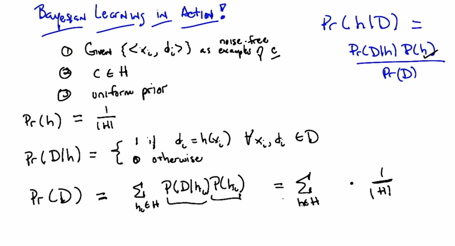
C: Okay Michael, so let’s see if we can actually use this as a way of deriving something maybe that we already knew. So I’m going to go through a couple of these because I I actually think, well, frankly I just think it’s kind of cool. But, I I’m hoping I can convince you it’s sort of cool too and that we get something out of it. Okay, so let me set up the word, I’m going to set up a a problem, and it’s going to be a kind of generic problem, and I’m going to see what we can get out of it, okay? So this is machine learning, so we’re going to be given a bunch of data, so there are three assumptions that I’m going to make here. The first is that we’re going to be given a bunch of labeled training data, which I’m writing here as x sub i and d sub i, so x sub i is whatever the input space is, and d sub i are these labels. And let’s say, it doesn’t actually even matter what the labels are, but let’s say that the labels are classification labels. Okay?

M: Hm.

C: All right. And furthermore, not only we’re given this data as examples drawn from some underlying concept c, but they’re, in fact, noise-free. Okay? So they’re true examples that tell you what c is. Okay?

M: Mm-hm.

C: So I’m going to say, in fact, let me write that down because I think it’s important. They’re noise-free examples. Okay.

M: Like di equals c of xi.

C: That’s right, for all xi. So, the second assumption, is that the true concept c, is actually in our hypothesis space, whatever that hypothesis space is. And finally, we have no reason to believe that any particular hypothesis in our hypothesis space is more likely than any other. And so, we have a uniform prior over our hypotheses.

M: So it’s like the one thing we know is that we don’t know anything.

C: That’s right. So, sometimes people called this an uninformative prior because you don’t know anything. Except of course I’ve always thought that’s a terrible name because its a completely informative prior. In fact its equally as informative as every other prior in that it tells you something that all hypotheses are equally likely. But that’s

M: I thought it was called an uninformed prior.

C: Is it? So its just an ignorant prior is what you’re telling me. Yeah.

M: Okay. Well, then maybe that’s the problem. I just always had a problem with it because people keep calling it uninformative and the really mean uninformed. Okay. In any case, so these are our, these are our assumptions. We’ve got a bunch of data, it’s noise free, the concept is actually in the hypothesis base we care about and we have a uniform prior. So we need to compute the best hypothesis. So given that we want to somehow compute the probability of some hypothesis given the data, right? That’s just Bay’s Rule. So, Michael, you’ve got the problem right?

C: Yes.

M: [LAUGH] okay. So in order to compute the probability of a hypothesis given the data, we just need to figure out all of these other terms. So let me just write down some of the terms and you can tell me what a you think the answer. Okay.

C: Well, what was the question?

M: The question is, while we want to compute some kind of expression for the probability of a hypothesis given the data. So given some particular hypothesis, I want to know what’s the probability of that hypothesis given the data, okay?

C: Yeah.

M: Okay, you got the setup. So, we’re going to compute that by figuring out these three terms over here. So, let’s just pick, one of them to do. Let’s try the prior probability. So Michael, what’s the prior probability on H?

C: Did we say that it was a finite hypothesis class?

M: It is a finite hypothesis class.

C: Then it’s like, one over the size of that hypothesis class because it’s uniform.

M: Exactly right, uniform means Exactly that. Okay so we’ve got one of our terms, good job. Lets pick another term. How about the probability of data given the hypothesis. What’s that?

C: The probability, so I guess noise free, and we know that it’s noise free so it’s always, so they’re always going to be zeros and ones.

M: Mm-hm.

C: So, and it’s going to be a question of whether or not the data is consistent with that hypothesis. Right, if the labels all match.

M: Right.

C: What we expect them to be if that really were the hypothesis, then we get a one, otherwise we get a zero. That’s exactly right. So let me see if I can write down what I think you just said. The probability of the data, given the hypothesis, is, therefore one if it’s the case, that the labels And the hypothesis agree for every single one of the training exercises. Right?

M: Yep

C: Is that what you said? Good. And if any of them disagree, then the probability is zero. So that’s actually very important. It’s important to, to understand exactly what it means for, to have the probability to get a hypothesis, as we mentioned before. That the English version of this is, what’s the probability that I would see data with these labels in a universe where H is actually true. Which is different from saying that H is true or H is false. It’s really a common about the labels that you see on a data. In a universe, where H happens to be true.

M: Okay, but you know, it’s occurring to me now that you wrote that down, that we’ve talked about this idea before.

C: When?

M: Well, so, like there’s a shorter way of writing that. Which is D of H equals one if H is in the version space of D.

C: Huh, that’s exactly right, that’s exactly right. So, in fact, that will help us to compute the final term that we need, which is the probability of seeing the data labels. So, how do we go about computing that? Well, it’s exactly going to boil down to the version space as you say, let me just write out a couple of steps so that it’s pretty Kind of easy to see. It’s sometimes easier in these situations to kind of break things up. So, the probability of the data sort of formally, is equal to just this. So we can write the probability of the data as being, basically, a marginalized version of the probability of the data given each of the hypotheses times the probability of the hypotheses. Now, this is only true in a world where our hypotheses are mutually exclusive. Okay so let’s assume we are in that world because frankly that’s what we always assume and this little trick is going to workout for us because we are going to get to take advantage of two terms that we already computed naming the probability that the data given the hypothesis and the probability of a particular hypothesis so we know that prior probability of a hypothesis is right, its just one over the side of the hypothesis space and how am I going to substitute in this equation for the probability of the data given the hypothesis?

M: So, I don’t know. I would write that differently. I mean, it’s basically it’s like the indicator function on whether or not HI is in the virtual space of D.

C: Right, that’s exactly right. So in fact this is not a good way to have written it. Let’s see if I can come up with a, a good notational way of doing it. Let’s say, for every hypothesis that is in the version space of the hypothesis space given the labels that we’ve got. Okay? How’s that count?

M: Okay.

C: So rather than having to come up with an indicator function, I’m just going to define vs as the subset of all those hypotheses that are consistent with the data.

M: Yeah exactly

C: Okay, and so whats the probability of those?

M: One It’s one and it’s zero otherwise, so then, we can simplify the sum and it’s simply what? ?

C: The sum of the one, ooh! The one of each doesn’t even depend on the hypothesis.

M: mm-mh!

C: I see wait I don’t see oh yes I do, I do its one over the size of version space. No its the size of the version space over the size of the hypothesis space.

M: That’s exactly right. Basically for every single hypothesis in the version space we’re going to add one and how many of those are? Well the size of the version space number of those. And multiply all that by one over the size hypothesis space, and so the probability the data is that term. So now we can just substitute all of that, into our handy dandy equation up there, and let’s just do that. So the probability of the hypothesis given the data, is the probability of the data given the hypothesis Which we know is one for all those that are consistent, zero otherwise. The probability of the prior probability over the hypothesis is just one over the size of the hypothesis space, and the probability of the data is the size of the version space Over the size of the hypothesis space which, when we divide everything out, is simply this. Got it?

C: Got it.

M: So, what does that all say? It says that, given a bunch of data, your probability of a particular hypothesis being correct, or being the best one or the right one, is simply uniform over all of the hypotheses that are in the version space. That is, are consistent with the data that we see.

C: Nice.

M: It is kind of nice. And by the way, if it’s not consistent with it, then it’s zero. So, this is only true for hypotheses that are still in A version space and zero otherwise. Now notice that all of this sort of works out only in a world where you really do have noise free examples, and you know that the concept is actually in your hypothesis space and, just as crucially that you have a uniform prior for all the hypotheses. Now this is exactly the algorithm that we talked about before right. We talked about before what would we do. To kind of decide whether a hypothesis was good enough in this sort of noise-free world. And the answer we came up with is you should just pick one of them that’s in the version space. And what this says is there’s no reason to pick one over the other from the version space. They’re all equally as good or rather equally as likely to be correct.

C: Yeah, that follows.

M: Yeah. So there you go. So it turns out you can actually do something with this. Notice by the way that we did not pick a particular hypothesis space, we did not pick a particular form of our instance space, we did not actually say anything at all about exactly what the labels were other than that they were labels of some sort. The strongest assumption that we made was a uniform prior, so this is always the right thing to do. At least in a Bayesian sense in a world where you’ve got noise free data, you have to find that hypothesis space, and you have uniform priors. Just pick something from the consistent set of hypotheses.

Quiz: Noisy Data

scribble

• The probability that you get one of those multiples is

• Why was bayes rule not used or applied here?

  • We are calculating the probability of Data given h? So, we simply use the probability rule?

• You should not be looking for patterns in the column (mistake I made).
• These are independent, so the probability of all these happening is the product.

\[1 / 2^k\]

slides

transcripts

C: Alright, Michael, I got a quiz for you, okay?

M: Sure.

C: So, in the last example we had noise free data. So I want to think a little bit about what happens if we have some noisy data. And so I’m going to come up with a really weird, noisy model. But hopefully it illustrates the point. Okay.

M: Sure.

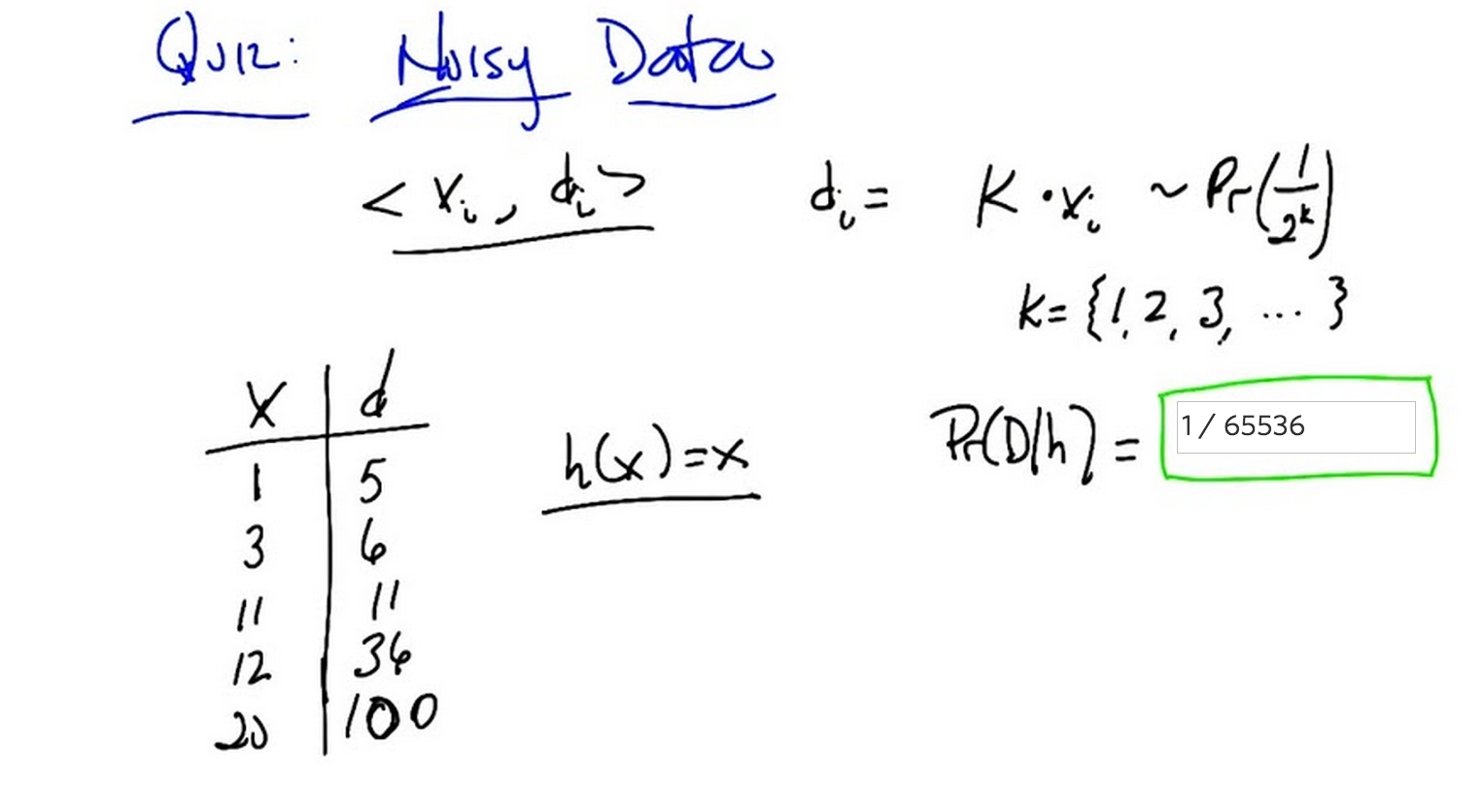
C: Okay so i got a bunch of training data, its x of i d of i and here’s how the true underline process sort of works. So give us some particular x of i, you get a label which is d of i which is equal to k times x of i where k is some number So one of the counting numbers, one, two, three, four, five, six, seven, eight, and so on and so forth. And the probability that you actually get anyone of those multiples of x of i is equal to one over two to the k. Now why did I choose one over two to the k? Because it turns out that the sum of all those two to the k’s from one through infinity happens to equal to one. So it’s a true probability distribution.

M: Hmm, okay.

C: So it’s just a neat little geometric distribution. So, you under understand the setup so far?

M: I think so, so before hypothesis were producing answers then we looked for them to be exactly in the data. Now we’re saying that the hypothesis produces an answer, and it gets kind of smooshed around a little bit before it reappears in the table, thats the noisy part.

C: Right, so you, you’re not going to be in a case now, that if the hypothesis disagrees with the label it sees. That in fact that means no it can’t possibly be the right hypothesis because there’s some stochastic process going on that might corrupt your output label, if you want to think of it as corruption, since it’s noisy. Okay?

M: Okay, yeah sure.

C: Alright?

M: Okay, so here’s a set of data that you got. Here’s a bunch of x’s that, that make up our training data one, three, 11, 12, and 20. For some reason they’re in ascending order. And the labels that go along with them are five, six, 11, 36, and 100. So you’ll notice that they’re all multiples of some sort of the input x. Okay?

C: Alright.

M: Now I have a candidate hypothesis. H of x which just returns x. That’s kind of neat. So it’s the identity function. So, what I want you to do is to compute the probability of seeing this particular data set in a world where that hypothesis, the identity function, is in fact true.

C: The identity function plus this noise process.

M: Yes.

C: And one other question quickly this, this noise process is supplied independently to each of these inputs, outputs, pairs?

M: Yes, absolutely.

C: Okay, then, yeah, I think I can do that. Uh-huh.

M: Okay, go.

Answer

C: Okay, Michael. You got the answer?

M: Yeah, I think, well I can work through it, I don’t actually have the number yet.

C: Okay, let’s do that.

M: So, alright, so in a world where.

C: In a world where.

M: Where this is the hypothesis that actually matters. We’re saying that X comes in, the hypothesis spits that same X out. And then this noise process causes it to become a multiple. And the probability of a multiple is this one over two to the case. So, the probability that that would happen from this hypothesis. for the very first data item. The one to five, would be

C: Okay. How do you, how’d you figure that out?

M: Cause the k that we would need the multiplier would have to be five. And so the probability for that multiplier is exactly one over two to the five which is one 30 second.

C: Okay.

M: And so then I would use that same thought process on the next one which says that it is doubled and the way that this particular process would have produced a doubling would be if with, with probability a quarter.

C: Uh-hm.

M: And, the next data element would have been produced by this process with probability at half, because it’s k will be 1, and 1 over 2 to the k would be half,

C: Okay, I like this.

M: Right? The next one will be an 8th, because its tripled,

C: Uh-hm.

M: And the last one is also a multiplier of 5, just like the first one, so that will be one thirty second as well,

C: Mm-hm.

M: Alright but now we need to assign a probability to the whole data set, and because you told me it was okay to think about these things happening independently, the probability that all these things would happen is exactly the product.

C: Right.

M: So I’ll multiply a 32nd and a quarter and is 7 plus 1 is 8. Plus another is 65,536. So it should be 1 over, oh you already wrote it. 65,536. Yea that.

C: Yes that’s absolutely correct Michael. Well done. Okay so, that’s right, but you did it with a bunch of specific numbers. Is there a more generic Is there a general form that we could write down?

M: Yeah, I think so, we’re doing something pretty regular once I fell into a pattern. So, I took the D, and divided by X, so D over X tells me that the multiplier that was used, so that’s like, the K.

C: So. D over x gave you the k.

M: And it was one over 2 to the that.

C: Okay, so one over 2 to the that.

M: And it was then the product of, of that quantity for all of the data elements, so all the i’s. So product over all the i’s of that.

C: Okay.

M: But we have to be careful because If it was the case that for any of our xi’s the d wasn’t a multiple of it, that can’t happen under this hypothesis and the whole probability needs to go to zero.

C: Right.

M: So they all have to be divisible otherwise all bets are off.

C: Okay, so in other words if d of i mod x of i is equal to zero and this formula holds and it’s zero otherwise.

M: Exactly.

C: Okay. Sounds good. Okay, great Michael. So that’s right and that was exactly the right way of thinking about it. And now, what we’re going to do next, is we’re going to take what we’ve just gone through. This sort of process of thinking about, how to generate data labels. for, you know, noisy cases and we’re going to apply to it what I think you will find will be a pretty cool derivation. Sound good?

M: Awesome!

C: Excellent.

Return to Bayesian Learning

scribble

• Lots of details in this chapter.
• Need to take multiple slides.
• Zero mean. What does it even mean?
• Variance.
• iid?
• Error representation is via normal distribution.
• Minimizing the sum of squared errors.
• Gaussian Noise.

slides

transcript

C: Okay Michael, so that was pretty good with the quiz. I want to do another derivation and I want you to help me with it, okay?

M: Hm. Cool.

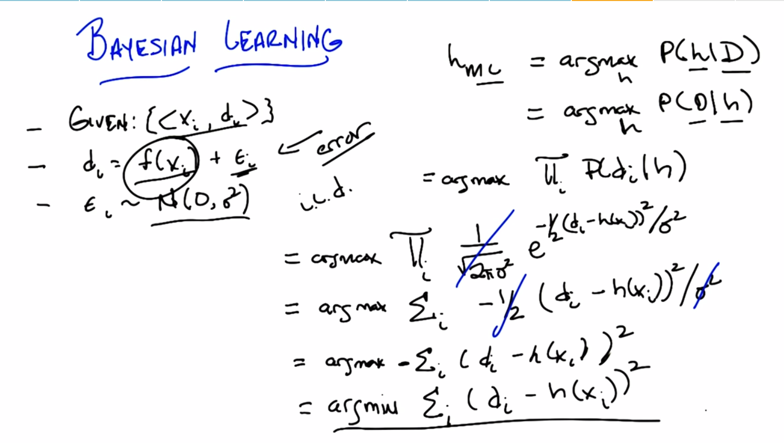
C: Okay, so Michael, we have a similar setup to what we’ve had before. We’re given a bunch of training data, XI inputs and DI outputs. But this time we’re dealing with real valued functions. So the way DIs are constructed is there’s some Deterministic function f, that we pass the fs through. And that gives us some value. And that’s really what we’re trying to figure out. What is the underlying f? But to make our job a little bit harder, we have noisy outputs. So, for every single DI that is generated, there’s some small error, epsilon that is added to it. Now, this particular error term, is in fact drawn from a normal distribution with zero mean and some variance. We don’t know what the variance is. It’s going to turn out. It doesn’t actually matter. There’s some variance going on here. The important thing is that there’s zero mean. So, you got it?

M: And it’s important that it’s probably the same variance for all the data.

C: That’s right, in fact, each of these epsilon sub i’s are drawn iid.

M: And is that f, are we assuming it’s linear?

C: Nope, we’re not assuming that it’s linear.

M: Okay.

C: It’s just some function.

M: All right, I’m with you.

C: Okay, so you got it?

M: Yep.

C: All right. So, here’s my question to you. What is The maximum likelihood hypothesis.

M: Do we know f? Can I just say f?

C: No, we don’t know f. All we see are x sub i’s and d sub i’s. But we know there is some underlying f. And we know that it’s noisy, according to some normal distribution.

M: I don’t know how I would find that.

C: Well let’s try to walk it through. So. We know how to find the maximum likelihood hypothesis, at least we know an equation for it. The maximum likelihood hypothesis is simply the one that maximizes this expression.

M: Right. That was when we assumed a uniform prior on the hypotheses.

C: Exactly. And so we, this is sort of the easiest case to think about Where it turns out that finding the hypothesis that best fits the data is the same as finding a hypothesis that describes

the data the best. If you make an assumption about a uniform distribution, or a uniform prior. Okay, so. This is all we have to do now is figure out what we’re going to do to expand this expression. So what do you think we should do first? The probability of the data given the hypothesis. Right. So each we assumed IID.

M: Mm-hm.

C: You actually helpfully even wrote that down. So we can expand that into the product over all the data elements of the probability of that data element given the hypothesis. And x. M: Okay, so let’s do that, Michael. Let’s write that out. So, finding the hypothesis that maximizes the data that we see, as you point out, is just a product over each of the independent data that we see. Or datums. So that’s good. That’s one nice step. So we’ve gone from talking about all of the data together to each of the individual training data that we see. So what do we do next? What is the probability of seeing one particular P sub i, given that we’re in a world where H is true.

C: So okay, given that H is true that means whatever the corresponding xi is, if we push that through the f function, then the di is going to be F of XI plus some error term soI guess if we took di minus F X I, that would tell us what the error term is and the we just need an expression for saying how likely it is that we get that much error.

M: Right, so, what is the expression that tells us that?

C: I’m guessing it’s something that uses the normal distribution, it probably has an E in it.

M: [LAUGH] I think that’ s absolutely right. So, let’s be particular about what you said. So, when you say that we should push it through F of X, let’s be clear that that’s basically what H is supposed to be. Our goal here is, given all of this training data, lets recover what the true f of x is. And that’s what our H is. Each of our hypotheses a guess about what the true underlying deterministic function F is. So, if we have some particular labels, some particular value D sub I that is at variance with that. What’s the probability of us seeing something that far away from the true underlying F. Well, it’s completely determined by, the noise model. And the noise is a Gaussian. So, we can actually write down Gaussian. Do you remember what the equation for a Gaussian is?

C: Yes. It’s exactly something that has an E in it.

M: That’s right. So I’ll see, I’m going to start writing it and you see if you remember any of what I’m writing down.

C: E to the…

M: No.

C: Okay, good.

M: It’s 1 over.

C: E to the.

M: No.

C: Okay.

M: Square root of, it’s, it’s coming back to you now. 2 pi sigma squared.

C: Okay.

M: Times…

C: I was going to put that in after.

M: Oh, okay. So now you get your E, so E to the what?

C: It’s going to be the value, which, in our case, is, like, H of XI minus DI.

M: Yeah. And then I feel like, we probably square that?

C: Yep.

M: And then we divide by sigma squared?

C: right.

M: Really?

C: Yeah.

M: Sweet!

C: And you’re missing one tiny thing.

M: There needs to be another two.

C: Yes. And in fact it’s minus one half.

M: Got it.

C: So, this is exactly the form of the Gaussian in the normal distribution. And what it basically says is the probability me seeing some particular point, in this case DMI. Given that the mean is H of X. Which is to say that’s the underlying the function. Is exactly this expression. E to the minus one half, of the distance from the mean, squared, divided by the merits. Okay. And that’s just, you either remember that or you don’t. But that’s just the definition of a Gaussian. So that means the probability of us seeing the data is the product of the probability of us seeing each of the data items. And that’s just the product of this expression here. Good. Now, we need to simplify this. We could stop here because this is true, but we really need to simplify this and I think it’s pretty… Not to hard to do. It’s pretty easy.

M: Mm..hm.

C: What kind of trick do you think we would do here to simplify this?

M: So, first thing I would do is, noticed that the 1 over square root 2 pi sigma square doesn’t depend on i at all, and maybe move it outside the pi but then realize, well, actually since we’re doing an argmax anyway, it’s not going to have any impact at all. [CROSSTALK] I would just like cross that baby out.

C: I like that. No point in keeping it. All right, now I’m hoping that the other sigma squared we can make that go away too. So I’m tempted to just cross it out, but I’d rather, I’d be much more happy if I had a good explanation for why that’s okay.

M: Well, so what’s the normal trick, so we’re trying to maximize the function, right? What you just said is we can get rid of this particular constant expression because it doesn’t affect the max. What’s making it hard for you to get rid of the sigma squared here is that it’s being passed through some exponential and you can’t remember off the top of your head what clever work you can do with constants inside of exponentials. So it would be nice if we could get rid of the exponential.

C: Very good. So because log is concave.

M: No, because it’s monotonic.

C: um-hm. We can take the log of the whole shabang. So this is going to be equal to the argmax of the sum of the log of that expression, which is going to move the thing to the outside and the log of E, so that’s going to be good, so it’s going to be the sum of the superscript thing, the power.

M: Right. So let’s write that down. Okay, so just to be sure that that was clear to everybody, let’s just point out that we basically took the log of both, the natural log of both sides, and so we said, instead of trying to find the maximum hypothesis or the maximum likelihood hypothesis by evaluating this expression directly, we instead evaluated the log of that expression. And as you’ll recall from intermediate algebra, the log of a product is the same as the sum of the logs, and the log of E to something is just that thing.

C: As long as we do natural log.

M: As long as we do natural log when we have E. If we were doing something to the, 2 to the power of something, we’d want to do log base 2. Okay.

C: Got it. And you said to do it to both sides but we really didn’t need to do it to both sides we just needed to do it inside the things we taking the argmax.

M: That’s correct. Okay, so we’ve got here. So, is there any other simplifying that we can do.

C: Yeah, yeah now it seems much clearer so the. The negative one half divided by sigma squared all can move outside the sum because it doesn’t depend on I at all.

M: Right. And then the sigma squared you said that before you said that that wasn’t going to turn out to matter. Both sigma squares ended up, you know, getting tossed into the rubbish heap.

C: That’s right.

M: And I want to be careful with the negative sign. Like I feel like the half can go and the sigma square can go but the negative has to stay.

C: You’re right. The half can go. And the sigma squared can go. So that leaves us with this expression. So I’ve taken, gotten rid of the one half, like you suggested. Got rid of the sigma squared like you suggested, and I moved the minus sign outside of the summation. And I’m left with this expression.

M: I have a thought about getting rid of that minus sign.

C: Well how would you get rid of a minus sign?

M: So the max of a negative is the min. Right, so we can get rid of the minus sign by just simply minimizing instead of maximizing that expression. We end up with this expression.

C: Nice. That’s much simpler than where we started. The e is gone.

M: It’s much simpler. We got rid of a bunch of e’s. We got rid of a bunch of turns out extraneous constants. We got rid of multiplication. We did a bunch of stuff, and we ended up with this.

C: You know, we got rid of two pis. It’s kind of sad I would like some pie.

M: Mm, I wonder what kind of pie it was?

C: Pecan pie?

M: [LAUGH]

C: Okay, so we got this expression, and that’s kind of nice on your own you say, but actually it’s even nicer than that.

M: What?

C: What does this expression remind you of Michael?

M: The Sum of Squares.

C: This is exactly it. This is, in fact. The sum of squared error, which is awesome.

M: Yeah, whoever decided it would be a good idea to model noise as a Gaussian was really on to something.

C: Mm-hm. Now, think about what this means, Michael. We just took, using Bayesian Learning, a very simple idea of maximizing a likelihood. We did nothing but substitution, here and there. With the noise model. We got rid of a bunch of things that we didn’t have to get rid of. We cleverly used the natural log. Notice that the minus sign can be taken away with the min. And, we ended up with some of squared error. Which suggests that all that stuff we were doing with back propagation. And, all these other kinds of things we’re doing with receptrons is the right thing to do. Minimizing the sum of square error, which we’ve just been doing before. Is in fact the right thing to do according to Bayesian learning.

M: Right in this case meaning meaning what a Bayesian would say.

C: Meaning what a Bayesian would say which I believe is sort of right by definition. More importantly here it is.

M: They certainly believe it.

C: Well, they, they do frequently.

M: Oh! I see what you did there.

C: No one will get that but, but us. Anyway, the thing is this is the thing you should minimize if you’re trying to find the maximum likelihood hypothesis. Now, I just want to say something. That is beautiful. Absolutely beautiful. That you do something very simple like finding the maximum [UNKNOWN] hypothesis and you end up deriving some of squared errors.

M: So, just to make sure that I’m understanding. because I see some beauty here, but maybe not all of it. We didn’t talk about what the hypothesis class here was. Right, so, if you don’t know what the hypothesis class is… You’re, you’re kind of stalled at this point, but if we say the hypothesis class is say linear functions.

C: Mm-hm.

M: Then, what we’re saying is we can do linear regression, because linear regression is exactly about minimizing the sum of the squares, right? So linear regression comes popping out of this kind of Bayesian perspective just like that, so is, is that part of what makes it so cool?

C: That is part of what makes it cool, but I just think more generally about gradient descent right? The way gradient descend works is you take a derivative by stepping in this, in this space of the air function, which is sum of squared error.

M: I see, so you get gradient descend too.

C: Yes, you get all of the stuff that people have been doing. Now, there’s a piece of beauty there, which is that we derived things like gradient descend and linear regression, all of the stuff we were talking about before and we have an argument. For why it’s the right thing to do at least in a Bayesian sense. But there’s an even deeper beauty here, which is tied in with ugliness, which is the reason this is the right thing to do, is because of the specific assumptions that we’ve made. So what were the assumptions that we made? We assumed that there was some True deterministic function that was mapping our x’s to our in this case our d’s and that they were corrupted say transmission error or line noise or however you want to think about it. They are corrupted by some noise that has a very particular form. Uncorrelated, independently drawn, Gaussian noise, with mean zero. So the less pretty way of thinking about it is. Whenever you’re trying to minimize the sum of squared error, you are in fact assuming that the data that you have has been corrupted by Gaussian noise. And if it’s corrupted by some other noise, or you’re actually not trying to model determinance function, of this sort. And then you are in fact, possibly, in fact most likely doing the wrong thing.

M: I mean are there other noise models that lead to some other kinds of learning.

C: Sure, pick any other model in here that doesn’t look Gaussian at all, and you would end up with something else. I don’t know what you would end up with because. You know, you couldn’t do all these cute tricks with natural logs but yes, you would end up with something different. And one question you might ask yourself is well, if I try to do minimizing the sum of the squared errors, or something for which this model was not the right one, what sort of bad things might happen? Here let me give you an example, let’s imagine that we’re looking at this here, and our X’s are, I don’t know measurements of people. Okay? So height and weight. Something like that.

M: Mm-hm.

C: And in fact let’s make it, let’s make it let’s make it even simpler than that. Let’s imagine that our x is our height. And our outputs, our d’s, are say weight. And what we’re trying to learn is some kind of function from height to weight. Now, this doesn’t make a lot of sense to have a true [INAUDIBLE], but I’m trying to make a point here. So what we’re saying here is that we, we measure our height and then we measure weight. That there’s some simple relationship between them that’s captured by f. But, when we measure the weight, we get a sort of noisy version of that weight. Okay? That seems reasonable. But what’s not reasonable is we’re saying. Our measurement of the weight is noisy, but our measurement of height is not.

M: Because if the x’s are noisy, then this is not a valid assumption.

C: I see.

M: So, it seems to work a lot of the time and we have an argument for when it will work, but it’s not clear that this particular assumption actually makes a lot of sense in the real world. Even though in practice it seems to do just fine. Okay, got it?

C: I think so though I feel like if the error if you put an error term inside the f along with the x and f is say linear.

M: Mm-hm.

C: Then maybe it pops out and it just becomes another part of the noise term and, and it all still goes through. Like I feel lines are still pretty happy even with that.

M: No I think you’re right. Lines would be happy here because linear, I mean linear functions are very nicely behaved in that way. But of course, they’d have to be the same noise model in order for it to work the way you want it to work.

C: Yeah.

M: They’d have to both be Gaussian. They have to both have zero mean, right? And they’d have to be independent of one another. So your measuring device that gives you an error for your height would also have to give you an independent normal error for the weight.

C: Yeah. Though I feel like my scale and my yardstick actually are fairly independent. And they’re Gaussian? .

M: Oh mine is clearly Gaussian.

C: Yeah.

M: Yeah. Well at least they’re normal.

C: They’re normally are.

M: Mm-hm.

C: Okay good. So let’s move on to the next thing Michael. Let’s try one more example of this and, and then I hope that means you got it, okay?

M: Sure.

C: Beautiful.

Quiz: Best Hypothesis

scribble

• The derivation of the answer was very good.

slides

transcript

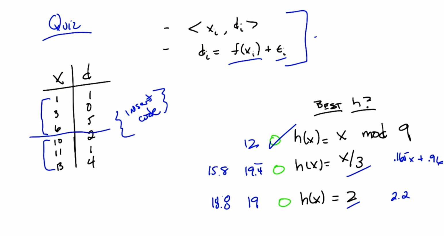
C: So before we go on to the next example, Michael, I wanted to do a quick quiz, just to make certain you really get what’s going on here. The, the sort of power of looking, using Bayesian learning. The, the main insight, I think, I, I want to drive home here, is something you said. Which is that, when we were doing regression before, when we were talking about the perceptrons, we actually had in our head a particular kind of function, a particular hypothesis class. In here with what been talking about with Bayesian learning, the answer tto finding to sum of squared errors was independent of the hypothesis class and only dependent upon the key assumptions that we were making, mainly that we had labeled the data with certain form, and that that data was generated by a process that took deterministic function and added some Gaussian noise to it. So, here’s the quiz. Here’s your training data. You’ve got a bunch of Xs and a bunch of Ds. These are the values that you have to learn. And I want you to tell me, which of these three functions over here, these three hypotheses is the best one under this assumption. Got it?

M: mod? Are we allowed to do that?

C: We are allowed to do that because

M: It’s just a function.

C: It’s just a function, man.

M: Interesting.

C: It’s just a function.

M: So we’ve got a linea-, a constant function, a linear function, and we’ve talked about those, but we’ve also got a mod function. alright, and we’ve got a uniform prior over these threes hypotheses.

C: Yup.

M: Okay. Yeah, I think I can do that.

C: Okay. Go.

Answer

C: Alright, we’re back, what’s the answer Michael?

M: So, you want me to work it through?

C: Sure.

M: So what I did first is I made it to, I extended the table that you had.

C: Okay.

M: To include each of these, the output for each of these three functions. What I’m basically, what I like to do is compute the squared error for each of these three functions on that data and then choose the one that has the lowest squared error.

C: Make total sense to me. Sounds good enough to be an algorithm. Aren’t you going to write out the table?

M: Well, I mean, I decided to do that, and then there was like one too many steps, and I just threw out my hand and just wrote this all down. Okay, so, we’ll just say” Insert code here”, because that’s what you did, that was the step.

C: And, what did your code tell you?

M: Well, let me start with the constant function, because that’s the easiest piece of code. So, I’m saying what’s the difference between each of the D values and two. Squaring it all and summing it up and I get 19. And I can do the same thing, instead of using two I use x over three take the difference of that to the D values and square that and I get 19 point [INAUDIBLE] four, four, four, four, four. Then I can do, right, so now at this point I’m rock and rolling. I can actually just substitute in my nine, and I get 12?

C: Not, not something-odd 12?

M: No, just 12, so the error’s 12. So that has the smallest error. So even though that’s sort of a crazy, like, stripy function right. Like, it increases linearly and then it resets at 9.

C: Mmhmm.

M: It actually fits the state of the best.

C: That is correct. Your code is correct, Michael. Well done. Well actually, looking at this data that sort of makes sense to me, right. Because if you look at the first three examples. Of the data, the outputs are very close. But the outputs of the next three are much bigger, and by doing a mod nine, what you effectively do is say, this is the identity function above this line. And then below the line, it’s as if I’m sort of subtracting nine from all of them, and that makes them closer together.

M: Hm.

C: And so it just happens to work out here. But surely that’s just because we came up with a bad constant function and a bad linear function. Do you think there’s a better linear function?

M: So I mean because it’s the squared error, we’re really just talking about linear regression.

C: Right.

M: So I can just run linear regression. So I get an intercept of 0.9588 And a, and a slope of 0.1647.

C: Okay

M: So that’s, so that’s my linear function of choice.

C: Okay, so that’s, what was, what was that again?

M: So x times, you know, it’s like a six, I guess, like 0.165 probably.

C: 0.165x

M: Plus

C: Mm hm.

M: Plus 0.959. So that’s our function, that’s our best linear function, the function that minimizes greater. So it better end up being, it better end up being less than 19.4, or I’m a liar.

C: Mm-hm.

M: And now I need to take the difference between that and D square it, and sum. 15.7.

C: Hm. So that gives you 15, I’m going to say 15.8. So that is better.

M: Yeah, so it’s better than the X over three, but it’s also worse than the mod nie.

C: Hm.

M: and the best constant function, has to be worse, because the linear functions include the constant functions as a subset, so this is, that 15.8 is. Is better than the best constant function too. Oh its easy to do though right? Because the best constant function is just the mean of the data.

C: What is the mean of the data?

M: 2.17.

C: huh two is pretty close.

M: Yeah that’s interesting.

C: Well that’s

M: Kind of in the middle of the pack I guess.

C: That sort of works right because two the error for two was actually lower than the error for x divided by three. And for what it’s worth the error for

M: Yeah, you’re not the [INAUDIBLE].

C: Yeah, eight would have been less than everything.

M: Okay. So, what have we learned here?

C: That sometimes you want to use mod.

M: Yeah.

C: If your data is weird. [LAUGH]

M: You have you have definitely modified my box.

C: Well I’m glad you found it mod. Hmm. [LAUGH] PUNS. Okay, good, so I think that was a good, that was, that was a good exercise. So I’m going to give you one more example of deriving something and then we’re going to move on.

M: Cool.

C: Okay.

Minimum Length Description

scribble

• log turns products into sums.
• length of the hypothesis is the number of bits needed to represent the hypothesis.

slides

transcript

C: All right, Michael. So I, all I have written up here for you is, are a maximum a posteriori equation, right? So the best hypothesis is the one that maximizes this expression. Nothing new, right? So I want to do a little trick, the same trick that you did before. So, you noticed that when we had E to the something, that we could use the natural log on E to get rid of everything. So I am going to try to do the same thing here. In the nat, why did the natural log work again?

M: Well, it’s the inverse of the E, but it let us turn products into sums.

C: Right. And the other reason it worked is because it’s a.

M: Oh, it’s monotonic.

C: Right, it’s a monotonic function and so it doesn’t change the argmax. So, I’m going to do the log of both sides here. But this time I’m going to do log base 2, for no particular reason other than it’ll turn out to help later. So, I’m just going to take the log of this entire expression, which, because it turns products into sums, gives me this. And by the way for those of you who haven’t noticed, I drew in a little bit of notation here. When you write just LG, it’s just log base 2. Okay, so, we agree that the answer to this equation and the answer to this equation is the same. And now I’m going to do one other little trick, exactly the trick that you used before. I’m going to change my max into a min, by simply multiplying everything by minus 1.

M: Okay, I don’t quite see where you’re going here.

C: But you agree that we haven’t changed the answer.

M: I agree that we haven’t changed the answer.

C: Okay. Do a log in there, do a minus sign in there that took us from a max to a min, but I haven’t changed the answer. Now, do you recognize anything about these expressions? I’ll give you a hint. Information theory.

M: Okay. So, information theory is usually entropy, which is like some of P log P stuff.

C: Right.

M: I’m not seeing that.

C: Well, there you, there’s your log and there’s your P.

M: Sure. It’s not P times that though.

C: That’s true. But we know from information theory, based exactly on this notion of entropy, that the optimal code for some event with probability P has length minus log base 2 of P. So, that just comes straight out of information theory. That’s where all the entropy stuff comes from. Okay. So, if we have some event that has some particular probability P of happening, the best code for it has this structure, minus log of P.

M: Okay.

C: So, if we take this fact that we know, and we apply it to here, what is this actually saying? This is saying that, in order to find the maximum a posteriori hypothesis, we want to some how minimize two terms that can be described as lengths.

M: Okay. I can see that.

C: So my question to you is, given that this definition over here, that an event with probability P has some length minus log P, what is this the length of?

M: So that would be the length of the probability of the data given the hypothesis.

C: Mm-hm.

M: And the length of the hypothesis, or the probability of the hypothesis.

C: Well no, it’s just the length of that hypothesis.

M: Oh, because the event is what has the length. Oh, I see. So it’s the length of the data, given the hypothesis, and the length of the hypothesis.

C: Right. So let’s write that out.

M: But I was just doing, like, pattern matching there. It’s not clear to me what a length of a hypothesis is. Hypotheses are functions. I don’t know how to take a tape measure to a function.

C: That’s fair. So this is the length of the hypothesis. Hypothesis. Right?

M: Yep.

C: So, you said you don’t know what that means. But, let’s think about that out loud for a moment. What does it mean to have a length of a hypothesis? That’s really sort of the number of bits you need to describe a particular hypothesis, right?

M: Okay.

C: Okay. And in fact, that’s exactly what it means. That’s why we use log base 2. So, if we want to minimize the length of a hypothesis, what does that mean, the number of bits that we need to represent the hypothesis?

M: The number of bits that we need to represent the hypothesis is, I guess, in some representation, or, so in this case I guess it would be some optimal representation. We are taking all the different hypotheses and writing them out. The ones that are more likely have a higher P of H, because that’s the prior. And those are going to have smaller lengths than the optimal code. And the ones that are less common are going to have longer codes.

C: Well, let’s make it more concrete.

Quiz: Shortest Length Tree

scribble

slides

transcript

C: So here are two decision trees, which one has the smallest link? Go.

Answer

C: Okay, Michael. Which of these two decision trees is smaller?

M: [LAUGH] The one on the right is smaller.

C: That’s exactly right because it’s easier, it’s, it’s easier to represent it in sort of almost any obvious way that you could think of. It has fewer nodes, so smaller decision trees, trees with fewer nodes, less depth, whatever you need to make it smaller, have smaller lengths than bigger decision trees. So that means that if all we cared about was the second term here. We would prefer smaller decision trees, over bigger decisions trees.

M: Which we do.

C: Which we do. Now what about this over here? The, what does it mean? So this is pretty straight forward. You got this right?

M: That the length of. Well, I mean guess what’s weird that you, you’re kind of moving back and forth between a notion of a prior, which is where the p of h came from and a notion of Well, you know, if we’re going to actually have to describe the hypothesis you’re going to have to write it down in some way, and this gives you a way of measuring how long it takes to write it down. But I guess what this whole derivation is doing is linking those two concepts, so that you can think about our bias for shorter decision trees as actually being the prior, right? Actually being the thing that says the smaller ones are more likely And vica versa, that when we think about things that are priors, that are assigning higher probability to certain things, it’s kind of like giving them a shorter description.

C: Right, so infact if you were to take this example literally here, that we prefer smaller trees to bigger trees, this kind of a bayesian argument for occam’s razor.

M: And pruning.

C: And pruning. Well, you, often use razors to prune, so it makes perfect sense.

M: Ok, so this is kind of straightforward, that basically smaller trees are smaller than bigger trees. It sort of makes sense. Now, what about this over here? What does it mean to talk about the length of the data given a particular hypothesis.

C: Uh…I could think of one interpretation there. So like, if the hypothesis generates the data really well, then you don’t really need the data at all, right? You just have…you already have the hypothesis. The data is free. Right? But if it deviates a lot from the hypothesis, then you’re going to have to have a long description of where the deviations are. So maybe it’s kind of capturing this sort of notion of how well it fits.

M: Right, that’s exactly right. So I like that explanation so let me write it down. So here we literally just mean something like size of h. But over here we are talking about, well sort of error right? if the hypo, if just exactly what you said if the hypothesis perfectly describes the data, then you don’t need any of the data. But lets imagine that the hypothesis gets all of the data labels wrong. Then when you send the hypothesis over To this person. This, this sort of person we’re making up who, trying to understand the Daden hypothesis. And you’re also going to have to send over what all the correct answers were. So, what this really is, is a notion of miss-classification error, or just error in general. If we’re thinking about regression. So, basically, what we’re saying is, if we’re trying to find the maximum Imposterior Hypothesis. We want to maximize this expression. We want to find the age that maximizes this expression. That’s the same as finding the age that maximizes the log of that expression, which gives you this. Which is the same as minimizing this expression, which is just maximizing this expression but throwing a minus one in front But these terms actually have meanings in information theory, the best hypothesis, the hypothesis with the maximum [UNKNOWN] probability is the one that minimizes error and the size of your hypothesis. You want the most simple hypothesis that minimizes your error. That is pretty much occam’s razor. What is important here In reality is that these are often traded off of one another. If I give a more complicated or bigger hypothesis, I can typically drive down my error. Or I can have a little bit of error for a smaller hypothesis. But this is the sort of fundamental tradeoff here. You want to find The simplest hypothesis that still explains your data, that is, minimizes your error.

M: Hm.

C: So this actually has a name, and that is the minimum description, and there have been many algorithms over the years that have tried to do this directly by simply trading off some notion of error, and some notion of size. And finding the tradeoff between them that actually works. Now, if you think about it for a little while Michael you’ll realize that yea this sort of makes sense at the hand wavy level at which I just talked about it. But, you do have some real issues here about for example units. So, I don’t know if the units of the size of the hypothesis are directly comparable to the counts of errors or you know sum of squared errors or something like that and so you have to come up with some way of translating between them… And some way of making the decision whether you would rather minimize this or you’d rather minimize that if you were forced to make a decision. But the basic idea is still the same here. That the best hypothesis is the one that minimizes error without paying too much of a price for the complexity of the hypothesis.

M: Wow. So I’ve been sitting here thinking about, so with decision trees, this notion of length feels… Like you could translate it directly into bits right like you actually had to write it down and transmit it, it makes a lot of sense. But then I was thinking about neural networks. And, and, and given that a fixed neural network architecture it’s always the same number of weights and they’re just numbers. So you just transmit those numbers. So I thought, hmmm, this isn’t really helping us understand and then it occurred to me that those weights, if they get really you’re going to need more bits to express those big weights. And in fact that’s exactly when we get over fitting with neural nets if we let the weights get too big. So like this gives a really nice story for understanding neural nets as well.

C: Right. That the complexity is not in the number of parameters directly but in what you need to represent the value of the parameters.

M: Wow.

C: So I could have ten parameters that are all binary, in which case I need ten bits. Or they could be arbitrary real numbers, in which case I might need, well, an arbitrary number of bits. That’s really weird.

M: Yeah, but the point here, Michael, I want to wrap this up. The point here is we’ve now used Bayesian learning to derive a bunch of different things that we’ve actually been using all along, and so again the beauty of Bayesian learning is that it gives you a sort of handle on why you might be making some of the decisions that you’re making.

C: It seems like this raises the theory question that you threw at me in a previous unit. Right. Which is like well so if it doesn’t really tell us anything we didn’t already know, how important is it?

M: Well in this case, I think it is important because it told us something that we were thinking and tells us in fact we were right. So now we can comfortably go out in the world minimizing some of squared error when we’re in a world where there is some kind of [UNKNOWN] transmission noise. We can go about trying to Believe Occam’s Razor because Bayes told us so. [LAUGH] Thanks to Shannon. And so on and so forth. We can do these things and know that in some sense, they’re the right things to do, at least in a Bayesian sense.

C: Okay, good. Now one more thing, Michael, I’m going to show you. Which is that everything I’ve told you so far is a lie.

Bayesian Classification

scribble

slides

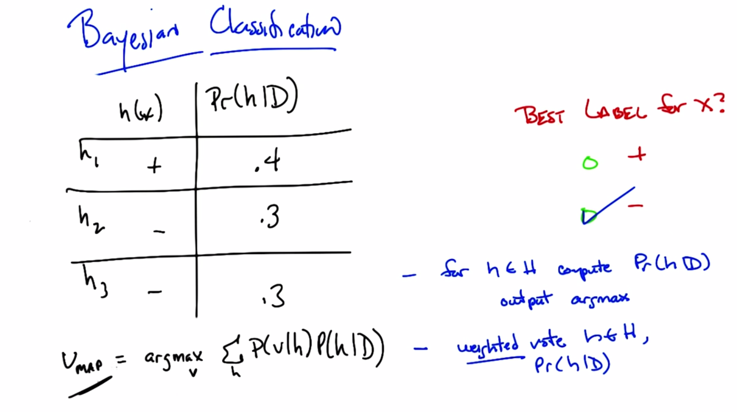
transcript

C: Okay, Michael, so here’s a quiz. Now it’s a pretty straightforward quiz. I just want you to use everything that you’ve learned so far. Okay, so you have three hypotheses. Let’s call them h1, h2, and h3, okay?

M: Mm-hm.

C: For the sake of argument. Here’s what each of these hypotheses Outputs or some particular x. h1 says plus. h2 says minus. h3 says minus. Okay?

M: Mm-hm.

C: Now here we’ve, already made it easy for you and we’ve computed the probability of, a particular hypothesis given some set of data. I’m not showing you the data but I’m showing you the answer for it. Okay? So the probability of h1 given the data is 0.4, h2 is 0.3, and h3 is 0.3. Got it? Wait hang on, so, okay, I see that corresponds here about this given data, what’s x?

M: x is some input, it doesn’t matter, just like it doesn’t matter what the date is.

C: [LAUGH] ‘Kay.

M: Just call it so that, that, x is x, okay? It’s just some object out in the world and each hypothesis labels it. Plus or minus.

C: ‘Kay.

M: Or can label it plus or minus. And H1 decides if for that X, it’s positive, and the other two hypotheses decide that it is, in fact, negative and H1 has probability that is the maximum a posterior probability h1 is .4, h2 is .3 and h3 is .3. So my question is, very simple. Using all of the magic we’ve done, this is just to make sure you’ve got it, Michael, I dunno, we’ve done a lot of derivations, we’ve walked away from somethings [LAUGH] we gotta make sure we get back to basics here. What is the best label for x? Is it plus, or is it minus? I see why this is tricky. Okay.

C: And go.

Answer

C: And we’re back. What’s the answer, Michael?

M: Okay, so it depends.

C: What does it depend on? I’ve given you everything. This is straightforward.

M: Well, so, okay, I guess. The here, so here’s what I’m seeing. So I’m, what I’m seeing is that hypothesis one is the most likely hypothesis.

C: It’s not just the most likely, it’s the most a posteriori.

M: Well, that’s what I mean by likely. Right, is the map hypothesis? It’s the maximum a posteriori hypothesis. So if we say, what is the label according to the map hypothesis? Boom, it’s plus.

C: Yes.

M: But, if we’re saying what’s the most likely label. So the most likely label is, is, we have to actually look over all the hypotheses and in a sense, let them vote. So the probability that the label is minus is actually 0.6, which is greater than 0.4, so if I had to pick, I would go with minus.

C: And you would be correct. So I did a little tricky thing here for you Michael. You’ve been complaining about my titles, because everyone said Bayesian learning and I changed the title here to Bayesian Classification.

M: Ohhh.

C: Because in fact the problem here, we’ve been talking about all along is, what’s the best hypothesis. But here. I ask you what’s the best label?

M: Hm. And exactly as you point out, finding the best hypothesis is a, is a very simple algorithm. Here I’ll write it for you because we did it before. For every H in hypothesis set, simply compute the probability that it is the best one, and then simply output max. That’s how you find the best hypothesis, but that’s not how you find the best label. The way you find the best label is you basically do a weighted vote for every single hypothesis in the hypothesis set, according to the weight being the probability of that hypothesis given the data.

C: Okay.

M: So the best, if you can only output hypothesis and use that hypothesis, in fact, you would say plus. But if you asked everyone to vote, just like we did with boosting, just like we did effectively with KNN and all these other kind of. Weighted regression techniques we’ve used before, you need to do the voting.

C: And I, and I feel like I could probably derive that using rules of probability. Right, because really what we want is we’re trying to maximize the probability of the label, given the data, and I think the probability laws would tell us that’s equal to some or all hypotheses of the hypothesis and the label given the data, which is, like, the probability of the hypothesis given the data, times the probability of the label given the hypothesis, and that’s what we did, we summed up. You know, the probability of the label given the hypothesis is either one or zero. That’s your left column. And then we’re summing up the probabilities that corresponding to the pluses. And we’re summing up the probabilities corresponding to the minuses and choosing the largest one.

M: So, this is what you just said written down as an equation. basically, the most likely value. Is the one that maximizes this expression. And this follows directly from Bayesian’s rule where now instead of trying to maximize the hypothesis given the data, you’re trying to maximize the value given the data. And I think it’s pretty straightforward to derive that but I’d like to leave it up to the students to do it on their own. Okay, so Michael, in some sense everything that I’ve told you before is a lie, in that I’ve led you down this path that somehow, finding the best hypothesis is the right thing to do. But the truth is, finding the value is what we actually care about. Finding a hypothesis is just a means to an end. And if we have a way of actually computing the probabilities for all the hypotheses, then we should let them both in order to find the best actual label or the best value for it.

C: Got it.

M: All right. Good.

Summary

scribble

• lot of fun.
• discovered an effective way to take online class with notes.

slides