Instance Based Learning

scribble

• It is mapping Chapter 8 in the machine learning book.

slides

transcript

C: Yeah, so I think that ,uh, what we’re going to end up talking about to day is kind of interesting, I hope. But it’s sort of different, and what I’m hoping is through this discussion Is that, we will be able to reveal some of the unspoken assumptions that we’ve been making so far, okay?

M: Unspoken assumptions, okay, that sounds like we should get to the bottom of that.

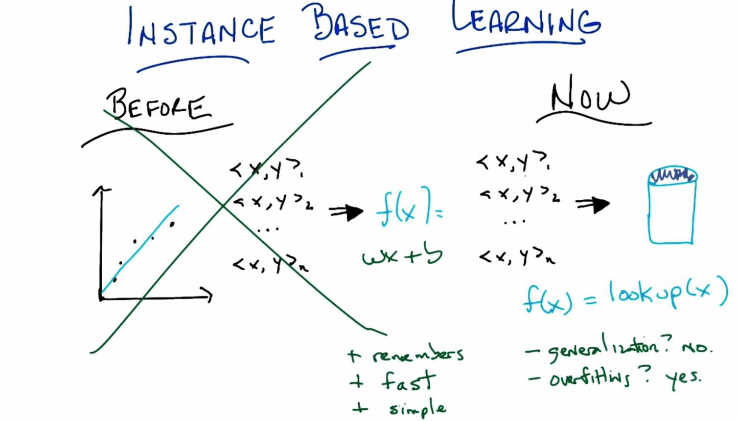
C: Yes, so let’s do that. So, just to remind you of what we have been doing in the past is what was going on with all of our little supervised learning tasks, right. We were given a bunch of training data ,labeled here as you know, x, y One, x, y two, x, y three, dot, dot, dot, x, y, z. And we would then learn some function. So, for example, if we have a bunch of points in a plane, we might learn a line to represent them, which is what this little blue line is. And what was happening here is we take all this data. We come up with some function that represents the data. And then we would throw the data away effectively, right?

M: Okay. Yeah, so black is the input here and then the two blue things are what get derived by the learning algorithm.

C: Right. And then in the future when we get some data point, let’s call it x, we would pass it through this function whatever it is. In this case, probably line. And that would be how we would determine answers going forward.

M: Yeah. That’s what we’ve been talking about.

C: Right. And in particular without reference to the original data. So. I want to propose an alternative and the alternative is basically going to not do this. So let me tell you exactly what I mean by that.

Instance Based Learning Now

scribble

• Not doing the approach of plotting the data and deriving a function from it.
• It has some advantages like, being simple, fast, but it cannot be generic and
• It has the problem of overfitting too.

slides

transcript

C: Okay, so here what I mean concretely by not doing this thing over here any more. So here what I’m proposing we do now. We take all the data, all of the training data we had, the x, y, 1, x, y, 2, dot, dot, dot, x, y, n and we put it in a database. And then next time we get some new x to look at, we just look it up in the database. And we’re done. None of this fancy shmancy learning. None of this producing an appropriate function like you know, wx+b, or what ever the equation of a line is. None of that fancy stuff anymore. We just stick in to the database. People written data base programs before. We’ll look it up when we’re done. Period.

M: I feel like you’ve changed the paradigm.

C: Yes, I am a paradigm changer. So what do you think?

M: It’s like, it’s like disruptive. It’s going to throw off the markets.

C: Yeah. It’s going to change everything. So, what do you think?

M: well, I mean, so there’s a bunch of really cool things about this idea. Which is why I’m excited. So one is it doesn’t forget, right? So it actually is very reliable. It’s very dependable, right, so if you put in an x, y pair you ask for the x you’re going to get that y back instead of some kind of crack potty, smooth version of it.

C: Right, that’s a good point. So we look at this little blue line over here, you’ll notice that say, for this little x over here, we’re not going to get back what we put in, so, it remembers, it’s like an elephant. Good.

M: So that’s kind of cool. Another thing is that there’s none of this wasted time, you know, doing learning. It just takes the data and it, and it’s, very rapidly just puts it in the database. So it’s fast.

C: It’s fast. It’s like. I like it when you say nice things about my algorithms. Okay. So it’s fast. Anything else, you can think of?

M: Yeah I can think of one more thing at least. Which is it’s simple.

C: That’s true. I am simple. I am simple and straightforward. I just need a few things to make me happy. Okay, so we’ve got three good things in remember stuff. So, you know, none of this little noisy throwing away information. It’s very fast, you just stick it in a database. Using your favorite database. And looking up is going to be equally as fast. And it’s very simple. There’s really no interesting learning going on here. So it’s the perfect algorithm when we’re done.

M: Okay. It feels like there’s more that we need to say though.

C: Like what?

M: In particular the way that you wrote this, F of X equals look up of X. If I give you one of the other points in between it will return no such point found. Which means it’s really quite conservative. It’s not willing to go out on a limb and say well I haven’t seen this before but it ought to be around here, instead it just says, I don’t know.

C: Mm. So the down side of remembering is, no generalization.

M: And I guess a similar sort of issue is that when you, when you call it memorization, it makes, it reminds me of the issues that we saw with regard to overfitting So, it bottles the noise exactly, it bottles exactly what it was given. So it’s going to be very sensitive to noise. So it’s kind of a yes and no.

C: So that’s a little scary and, and it can overfit in a couple of ways, I think it can over fit by believing the data too much that is literally believing all of it and what do you do if you have couple. What if you have you know a couple of examples that are all the same. I have got an x, shows up multiple times but each with a different y.

M: Oh, the same x. So the lookup would return two different things and this algorithm or whatever that you have described so far wouldn’t commit to either of them and it would just say, hey, here is both.

C: Yeah, that seems problematic.

M: Okay, alright. But I feel like, you know, you are going to to tell me, how to fix those things. So I wasn’t too worried.

C: Yeah, well, there is gotta be a nice way of fixing it. I think There’s sort of a basic problems here, which is that we’re taking this remembering and then looking up a little too literally, right? So I stick in the data, and I can get back exactly the data that I got, but I can’t get back anything that I don’t have, and that seems like something that we might be able to overcome if we’re just a little bit clever.

Cost of the House

scribble

• We based it off on nearest neighbor until we hit a point which was difficult to determine as there many conflicting nearest neighbor possibilities.
• This lead to K-Nearest Neighbor algorithm.

slides

transcript

C: Okay Michael, so let’s see if we can work together to deal with this minor triffle of a problem. You’ve observed my cool algorithm, okay. So, here’s some data, it’s a graph and you see here’s a y axis and here’s an x axis, and each of these points, represents a house, on this map, which I’m, I’m cleverly, using in the background. And, you’ll notice, that each of the dots is colored. I’m going to say that red represents, really expensive houses, blue represents, moderately expensive houses, and green represents, really inexpensive houses. Okay?

M: Okay, where is this?

C: Where is this? Oh, this is Georgia Tech, as you can tell because, it says Georgia Tech.

M: Oh, I see it now.

C: Okay. So, here’s what I want you to do. using machine learning. I want you to look at all of this data, and then I want you to tell me, for these little black dots, whether they are really expensive, moderately expensive or, or inexpensive. But I want you to do it using something like the technique that we talked about before.

M: Okay?

C: So let’s look at this little dot, over here. Which, by the way, I want to point out is this little black dot here by the US Post Office, underneath the rightmost e over here. It is not a point in our database. But I think by staring at this, you might be able to come up with a reasonable guess, about whether it is moderately expensive, expensive, or inexpensive.

M: Okay, yeah. I think, this is a helpful, example, because, now I see that it does kind of make sense, especially, in this context, to think of the geometric location, as actually being a very useful attribute for deciding how to label the new points. So, that black point that you’ve pointed out, is in the part of the neighborhood, that has a green dot in it. Like, the nearest dot to it, seems like a pretty good guess as to what, what the value of that house might be, so I’m going to guess green.

C: Yes, and I think ,you would be right. And I like the word that you used there. You talked about, its nearest neighbor, so I like that. I’m going to write that down. Neighbor, okay. So, I’m going to look at my nearest neighbor. Well let’s see if this works, for another point. Let’s look at another point, that’s near an, e, let’s see, the first e over here. This little black point, over here. What do you think? If I looked at my nearest neighbor, what what would I guess? M: Yeah, this one seems really clear. It’s, it’s surrounded by red. It’s in the red part of town.

C: So, you’re guessing, the output is then, purple?

M: No, I’m going with red.

C: Yes, and I think that that makes perfect sense. So, this is pretty cool. If I have a point that’s not in my database, but by looking at my nearest neighbour I can sort of figure out what the actual value should be. So, there we have solved the problem.

M: Yes, seems like a pretty good role.

C: Yeah, just look at your nearest neighbour and you are done. There is nothing else for you to do.

M: Yeah, except that you didn’t do all of the houses yet.

C: Okay, well, what did I miss?

M: The one in the middle and I’m wondering, if maybe you did that on purpose, because, this one has some issues.

C: What are its issues? Besides being too, near 10th Street?

M: well, yeah, apart from that it doesn’t really have any very close neighbors on the map. So the closest that you get, is maybe that red one?

C: Maybe.

M: But I would be really, I’d be very wary of just using that as my guess, because, it’s also pretty darn close to a blue point.

C: Yeah.

M: And also not so, far from the green point.

C: That’s a good point. So, this whole nearest neighbor thing doesn’t quite work, in this case when you got a bunch of neighbors that are saying different things. And they are kind of close to you. So, any clever way we might around this?

M: I would say, move the black dot.

C: No, no, no, no, we are not allowed that before.

M: No? Okay, right it seems, it seems, like it would be helpful.

M: No, no, they are federal laws against interesting.

C: I was going to say, yeah, so, alright. So short of that, we just need to look at a bigger context?

M: Ahh, that makes sense. So, you’re saying my little nearest neighbor thing, sort of worked, but the problem was I started out with examples that were, you know very clearly in a neighborhood and now I’m in a place where I’m not so sure about the neighborhood. So I should look at more of my neighbors than just the closest one.

Cost of the House Two

scribble

• Algorithm itself is simple, but lots of details are left out the designer of the algorithm.

slides

transcript

C: Okay, so, how many do you want to look at?

M: Well in this case I feel like I could draw the extended city block zone and capture I don’t know, five of the points.

C: Okay, let’s do it. So let’s find our five, our five nearest neighbors. So let’s see. This is clearly close, that’s one over here. I’d say this is close. I’ll say this one is close. This one’s close. None of the other blue ones are actually that close. And I’d say that’s the next closest one, so here are my little five points. That all seem relatively near. So what does that tell you? M: Well, I mean, it’s, it feels like it suggests that red is not a bad choice here.

C: Mm

M: It’s in a reddish part of town.

C: Yeah, I get that. So, so you think it’s a pretty, fair thing to bet that this should be red then?

M: Yeah I mean I think that if you were really asking me seriously I would wonder about that blue point to the right of the highway and whether that had any influence.

C: That’s pretty far away.

M: Yeah, it’s not that far away.

C: Well in Atlanta, once you cross highways you might as well be an infinite distance away.

M: Well so, okay, but. That’s a good point then. So, I guess I was interpreting your notion of distance as being, you know, like straight line distance on the map. But maybe that doesn’t make sense for this kind of neighborhood example.

C: Hm, no, that’s a good point. So, we’ve been talking about distance sort of implicitly. But this notion of distance. It’s actually quite important. So maybe distance is straight-line distance, maybe it’s as the crow flies. Maybe it’s driving distance. Maybe it has to take into account the fact that, when you cross highways in Atlanta, you’re typically moving into a completely different universe. These sorts of things matter.

M: Yeah. So I could imagine I don’t know, like Google Maps distance.

C: Right. Or how many paths can you get there and which is the shortest one given the traffic? There’s all kinds of things like that you could do. So. So that’s fair, that’s fair. But that just says that this, this distant, we have to be very careful what we mean by distance and that’s okay. But let’s just say for the sake of this discussion that these are the closest points by some reasonable measure of distance. So, in that world, would you be happy if you had to pick a single example? a single output, a single label of red, blue or green. Would you be happy picking red?

M: Yeah, I mean you know, not ecstatic, but okay.

C: That’s fair. So, I like this. So, we, we went from just picking our nearest neighbor to picking our nearest neighbors. What’s a good value you think we should stick to with neighbors? We started with one and that clearly wasn’t good. You picked, at least not in all cases and you came up with five. So what do you think? What if I’m going to call this algorithm something, what do you think five nearest neighbors? What do you think? What should I call it?

M: Five seems good. I mean I feel like that, that’s gotta be universal.

C: The number five?

M: Yeah.

C: Well it is in Atlanta but it might not be universal in wherever it is you are.

M: We’ll call it the Georgia Tech nearest neighbors.

C: That doesn’t seem like an algorithm that’s going to to be used very much.

M: Fair enough. All right. So what about, we could do as many nearest neighbors as is appropriate. Or maybe we should just make it a free parameter and call it K.

C: Ok, I like that. K nearest neighbors, so we’ll have K nearest neighbors. And we’ll pick our K numbers. Oh, and you said something fancy there, by the way. You said free parameter. I like that. We should, we should come back to that again. So we have an algorithm, k nearest neighbors. Which takes K nearest neighbors as a way of deciding how you’re going to label some query point here. And we’ve identified two parameters to the algorithm so far. K Which is the number of neighbors we’re going to use. And some notion of distance.

M: Oh, sure.

C: Which here we were kind of using in the sort of obvious way, but there might be other ways we might want to use distance here.

M: Yeah, like I could imagine if the houses, if, had additional features like how many Square footages they had.

C: Right, stuff like that. That would make perfect sense. We’re using distance here in a kind of in an overloaded sense, because this is something on a map. But really distance is a standard for similarity.

M: Similarity, good. It’s kind of standard for the opposite of similarity.

C: Well distance is just a kind of similarity, right? But in case of points on the map. Similarity, it sort of makes sense because as you said when we were talking about real estate, location, location, location matters. So, there, similarity really is kind of the inverse of distance. But in other ways, things like the number of veterans you have, whether you’re one on side of the highway or the other, the school district you’re in, things like that, are other things you might add as features or dimensions when you talk about similarity or distance. Okay, so I like this. I think we have a general algorithm now and I think it does a pretty good job of addressing the points you brought up. We no longer have to worry about overfitting as much, at least it seems that way to me. And we have a way of being a little bit more robust to this, you know, not having an exact data point in the database. So ,maybe we should turn this into an algorithm.

M: Yeah, let’s go for it.

K NN

scribble

slides

transcript

C: Okay, so what we have here, again, is pseudocode for our K-NN algorithm. And I’m sort of writing it as like, a function. So, you’re going to be given some training data D, that’s the little x, y points, x, y one, x, y, 2, x, y, 3, so on and so forth. You’re given some kind of distance metric or similarity function. And this is important because this represents the domain knowledge as I think we, we’ve already said. You get some number of neighbors that you care about, k, hence the k and n, which also, by the way, represents domain knowledge. Tells you something about how many neighbors you think you should have. And then are given some particular new query point and I want to output some kind of answer, some label, some value. So the K nn algorithm is remarkably simple given these things you simply find a set of nearest neighbors such that they are the K closest to your query point. M: Okay. I’m sort of processing this. So the data the capital D. Are those pairs and there’s a set of pairs?

C: Yes.

M: Ok. And k smallest distances. So this NN this is a set?

C: Yes.

M: And it’s consistent for all the elements in the data that are closest to the query point?

C: Yep.

M: And the so the query point is a parameter of that. Okay. Yeah. Alright. I think I. Oh. And then it’s, then the so it’s just return.

C: Yeah, so we haven’t figured out what to return. So there’s two separate cases we’ve been talking about so far. One is where, we’re doing classification, and one is where we’re doing regression. So, a question for you would be, what do you think we should when we’re doing classification? What will be a way of returning a proper label?

M: So you want to label, not a, like a weight on a label or something like that?

C: No. I want a label. You have to produce an answer. You have to commit to something Michael.

M: Alright. Can I commit to more than one thing?

C: Nope.

M: Okay. So I would say that a reasonable thing to do there would be. Did we get Ys associated with the things in NN?

C: Yep.

M: So I would go with they should vote.

C: I like that. I think that’s a good one, so we’ll simply vote and what does it mean to vote?

M: It means, let’s see, so feel like there would be a way to represent it in terms of NN, the set. Like do you want me to write it formally?

C: No.

M: Oh, then I would just say The closest point. Whichever yi is most frequent among the closest points wins.

C: Yeah. Right. So you want to find a, a vote of basically a vote of the yi’s, that are apart of the neighborhood set. And you take the plurality.

M: Plurality I see. So it’s whichever one occurs the most.

C: Right.

M: What if there’s ties?

C: It’s the mode. The mode. Right.

M: Right.

C: Mmmm. Ala mode.

M: What if they’re ties? That’s a good point. Well, if they are ties among the output, then you’re just going to have to pick one.

C: OK.

M: And there’s lots of ways you might do that. You might say, well, I’ll take the one. That is say, most commonly represented in the data period. Or I’ll just randomly pick each time, or any number of ways you might imagine doing that.

C: The one that’s first alphabetically.

M: The one that’s first lexicographically?

C: Hm.

M: What about in the regression case?

C: Okay. So in the regression case our y-is are numbers.

kM: Uh-huh. And we have the closest Yi’s, so we have a bunch of those numbers and it seems like [LAUGH] if you have a pile of numbers and have to return one, a standard thing to do would be to take the average, or the mean.

C: Yeah. Now let’s just simply take the mean of the Yi’s, and at least there, you don’t have to worry about a tie. That’s right. Though, I guess, you know. We didn’t really deal with the question of what happens if there’s more than k small. It’s, like, what if they’re all exactly the same distance? All n of them are exactly the same distance. So which are the k closest?

M: Well, there’s lots of things you could do there. I would suggest doing, is, take the, If you have more than k that are close, that are closest because you have a bunch of ties, in terms of the distance. Just take all of them. Get the smallest number greater than or equal to k. Okay.

C: That seem reasonable?

M: Yeah, I think that’s what college rankings do.

C: Actually, that is what college rankings do. That’s exactly what college rankings do. So, let’s do that. We know that college rankings make sense. [LAUGH]. Yeah, those are, they’re scientifically proven to be,

M: Youths. scary, scary to people in colleges.

C: That’s exactly right. So, here’s what we’ve got, Michael. So, all we do is we take the training data. We have some notion of similarity or distance. We have a notion of the number of neighbors that we care about. We have a query point, we find the K closest to one, you know breaking ties accordingly. And then we basically average in some way, in a way that make sense for classification, in a way they make sense for regression and we are done. It’s a very simple algorithm, but some of that’s because a lot of decisions are being left up to the designer. The distance metric. The number k, how you’re going to break ties. Exactly how you choose to implement voting. Exactly how you choose to implement the mean or the average operation that shows how to do here. And you could put a bunch of different things here and you end up in, completely, you could end up with completely different answer. Mm.

M: By the way, one thing that you might do, just to give you an example of how much range there is here. Is rather than doing a simple vote by counting, you could do a vote that is say, weighted by how far away you are. So we could have a weighted vote.

C: Uh-huh.

M: That might help us with ties.

C: That could help with ties. Yeah.

M:You could do a weighted average. Yes, right. So, you’re basically saying that the y values that correspond to x values that are closer to the query point have more of an influence on the mean.

C: Which makes some sense, right?

M: No, I think it makes a lot of sense!

C: So, how would you weight that? What would you do?

M: I would weigh it by the similarity.

C: Right, so well in this case, the similarity is we have a distance value similarity, so You would have to weigh it by something like one over the distance.

M: Oh I see. Okay. That seems like a hack.

C: Sure but it’s a hack that sort of makes sense.

M: Okay.

C: Okay. So anyway. Simple algorithm. Lots and lots of decisions to make here. All of which could in principle have a pretty big effect. And so, in order to see that, I want to do two quizzes that I hope get to heart of this and maybe give us a little bit of insight into how some of these decisions might matter on the one hand, and exactly just how simple or not simple this algorithm turns out to be. Okay?

M: Awesome.

Wont you compute my neighbors

scribble

slides

transcript

C: Okay Michael, I have two quizzes for you. Okay?

M: Yeah, yeah.

C: Here’s the first quiz, and here’s the way it’s set up. I want you to fill in the empty boxes of this table. Okay?

M: Ooh.

C: Got it.

M: There’s a lot of empty boxes.

C: There’s a lot of empty boxes.

M: Okay, but Okay, let me make sure I understand what’s going on here. So we’re looking at three different algorithms that are learning algorithms.

C: Yep.

M: There’s one One neural net

C: No

M: Okay, one nearest neighbor.

C: Mm-hm

M: K nearest neighbor and linear regression.

C: Yep

M: And for each one you want to know running time and space.

C: Mm-hm.

M: And this is on n points I assume, yeah, n sort, what does it mean for data points to be sorted?

C: So let’s assume we’re living in a world where all of our data points are you know in r one. Okay.

M: Oh okay that well that. That could be sorted.

C: That could be. Yeah that could be sorted. And that you know where going to be out putting some real numbers as well. So it points on a. On a number of lines. So to make things simple for you. I’m going to say that the points that you are given are already sorted.

M: Oh alright. It is just a scalar. So then a query point is going to come in. And then its going to be some value. And were going to have to find the nearest neighbor or do the regression or whatever.

C: Right.

kM: Alright now that’s for running time. Now for space, the space of what?

C: How much space you are going to have to do in order to accomplish your task. How much space you going to have to use in order to accomplish your task?

M: So this is kind of like the space that’s representing the class enviro. Or the regression. After training.

C: Yes. So actually that question about after training is important. You’ll notice I’ve divided each of these algorithms into two phases. There’s the learning phase. How much time it takes to learn. How much space you need to learn. Then there’s the query phase. When I give you some new value and you have to output and answer. What’s the running time for that and what are the space requirements for that? Okay? You got that?

M: Yeah

C: I want that for each one. Of these three algorithms.

M: Except for one nearest neighbor which the, it appears as though you filled in for me to get me started.

C: Right so just to get you started and make it easier for you know to know what I’m talking about. I’m talking about big O times here. Right. I’m not going to make you write out big O. Big O is implicit. So if we look at one nearest neighbor, and we ask well what’s the running time of learning? Well, it’s constant. Right? Because there’s no learning.

M: I see. You just take that sorted set of data points and you just pass it along through the query here.

C: Right. Now, you could say that” Well, I’m going to take the data points or I’m going to copy them into this database,” and so it’s linear. But let’s assume they already come in a database, or some data structure that you can use, okay?

M: Gotcha.

C: Okay, so now that actually brings us to a nice little question about how much space, learning takes here. And, well because you have to store those points, and keep them around. The space requirements are big O of N.

M: Yeah, that makes sense.

C: Okay, good. So given that as an example. Do you think your one example in your database. Mm, do you think you can use that to build up labels for all the rest of the phases of the different algorithms?

M: Yeah, I think so.

C: Okay, cool. Go for it.

Answer

C: Okay Michael, are you ready?

M: I am afraid so.

C: All right, which one do you want to fill out first?

M: Let’s just do them in order, so one nearest neighbor. You explained how the training works. We just take the assorted list, and leave it there.

C: Mm-hm.

M: And we have the classifier, or the aggressor itself has linear space, and now at query time, we need to find the nearest neighbor.

C: Which we could do by taking the query point and running through the whole list and seeing which one it’s closest. But because it’s sorted I think we outta be able to use binary search and, and in log time, find the closest point to the query.

M: That’s exactly right, you should be able to do that in log base two time. What if it weren’t sorted?

C: Yeah then, like I said, I think you could just scan through the whole list and that would be linear time and that’s not a big deal. M: Right, yeah, we could do linear time, but because I gave you a sorted list because, I’m so helpful, you can do it in log n time.

C: That was, that was very, very thoughtful of you.

M: It was I thought it through so what about on the, space side?

C: Alright, so the amount of space that you need to process its query is linear. We don’t need to take anything special, set aside space beyond a couple simple variables. And the data that we’re given, which we’ve already accounted for.

M: Right, so then why would it be linear, if we accounted for it?

C: Did I say linear? I meant constant.

M: Yes, yes, that’s right, constant. That’s what you meant. That’s what you said. That’s what happened.

C: It’s a good thing, this wasn’t being recorded, so we could verify one way or the other. M:It is a good thing, maybe we’ll look it up on Wikipedia, and it’ll say confusingly

C: Linear sometimes use to mean constant.

M: Constant. Yeah, that is pretty confusing.

C: Okay, what about k and n?

M: Alright, K and n. So k and n, so the training process, the learning process, is exactly the same, as it is for one year stamper, which is to say you do nothing and you pass all the data forward to the query processor. So it’s going to be 1 n.

C: That is correct, nice.

M: Now querying, seems like its a little more subtle. So we can find the single nearest neighbor in log and time.

C: Mm-mm.

M: Where we going to get the other K minus one? So, I’m pretty sure once we find the nearest neighbor we can kind of start doing a little spread out search from there until we found the k nearest neighbors.

C: Sure. So, you’re saying, you know, you’ve got these points. They’re already in a line, you find the nearest neighbor. You know the next nearest neighbors have to be within k of the points surrounding it, and so you can just move in either direction and pick them up as you go. Yeah, something like that.

M: Okay.

C: I think you can use the same algorithm that you used for merging lists, in merge sort, but here the lists actually corresponds to being to the left of the query point, and being to the right of the query point and they are both sorted in terms of their distance from the query point. Sure, yeah, I buy that.

M: So, so that ought to give us log n, plus k.

C: Okay, so, do we need to write the k?

M: I’m going to say yes, because, if k is on the order of n over 2, then it’s going to dominate. If k is on the order of log n, then it’s not going to dominate. Mm, that’s a good point. So, yeah, we’ll do k. I will point out that if k is on the order of n over 2 it will dominate and then really this is big O of n.

C: That’s right.

M: But if it’s on the order of log n, then it’s just log n plus n. So it’s just big O of log n. But, you’re right, so we should probably keep the k around because, we don’t know its relationship to n. Okay, fair enough. Okay, what about the space requirements?

C: We know one bit of relationship, it’s smaller than or equal to it.

M: That’s true.

C: Because that would be really weird, if I gave you ten data points and asked you for the 20 nearest neighbors.

M: That’s the sort of thing you would do.

C: It’s the sort of thing you would do, but then, it would be really confusing.

M: No, no, no, it’s the sort of thing you would do, again, let’s go to Wikipedia.

C: Confusingly, Twinny is sometimes [CROSSTALK]. [LAUGH]

M: Okay. So what about space?

C: Space, so, I don’t understand why, it would ever need more than constant space. So, so we’re going to zip around in that. If it does really badly, we can use K space. To kind of copy over what those, possible nearest neighbors are. But, we don’t need to keep track of them. We can just point to them in place, so it’s constant.

M: Okay, yea that’s true in fact, because, it’s sorted all you really need to know is the beginning and the ending. So, that’s two things that are constant. Okay, ao what about linear regression? Your favorite little algorithm thing that you did? When we talked about this before.

C: I do like linear regression. The learning in this case, is we are mapping real number inputs to a real number outputs. The way we are doing that is we are taking, its probably M X plus B sort of form [CROSSTALK]. We need to find the multiplier and the additive constant. Which in general doing a regression involves, inverting a matrix. But, in this case I think the matrix that we’re talking about is of constant size. So inverting is constant time. I think it’s as easy as basically just scanning through the list to populate a constant size matrix. So, I’m going to say order n.

M: Yep.

C: To process the data.

M: That is correct.

C: There’s probably a really nice algorithm for that.

M: Yeah, probably some kind of linear regression algorithm.

C: Yeah. No, I mean like the general linear regression algorithm is involves inverting a matrix.

M: Right.

C: Or something like it, something equivalent to it. But here because it’s all in scaler land, I think it’s simpler.

M: Yeah, I think that’s right. Okay so what about space?

C: All right, so space interpreted the data that you passed forward from the learning algorithm to the regressor is MX plus B. It’s just M and B, which are constant. There’s the two numbers.

M: Right, that’s 2, 2 is like 1, for large values [LAUGH] of 1, so it’s constant.

C: Yeah, All right, now at query time, you give me an X. I multiply, it by M and add B, so that’s constant time [CROSSTALK]. So,before the query cost was expensive and the learning cost was cheap. And now we’ve kind of swapped that around.

M: Yeah, we have, so space would be.

C: Space, oh, that you’re asking me?

M: Yeah.

C: Space for the query would be constant as well.

M: Right, exactly, so yeah, so you made a good point here. So earlier on, we had the situation where learning was fast, was constant, and querying was, you know, not as fast. It was, you know, probably logarithmic. But, in the regression case, learning was expensive and the querying was easy, so we swapped around, that’s exactly right. So, why would you care about that, well, let’s see, I’ll point out something, which is though, even though we swapped out what was expensive in terms of time and what wasn’t, you’ll notice it’s only logarithmic at query time for these first two but it’s linear for the learning time. Linear regression, so doesn’t that mean that linear regression is always slower and worse?

C: No really, because we only have to learn once, but we can query many, many times.

M: Right, right. So I guess if we query more than, you know, n times for example it’ll certainly be, worse overall. In terms of running time.

C: That’s right.

M: Okay.

C: Though, it’s interesting because like when I see numbers like this, my algorithm tells me that I should try to balance them a little bit more. It’s you can make learning essentially free and the other one you can make querying essentially free. Really you want to split those, somewhat evenly. Though it’s, not obvious to me how you would do that. Like, square root of n, learning time and then square root of n query time or something like that.

M: Yeah, but you did say something else that was important right? Which is that you only have to learn once.

C: Yeah, It’s true.

M: So, the balance you know, really depends on how often you’re going to do querying and exactly, what power it gives you. I mean, the trade off is really there. Don’t you think?

M: Yeah, I guess so. In the version where you just query ones.

C: Right.

M: Then the balance thing could be more interesting.

C: Sure, okay, cool. All right anything else you want to observe about this. Let’s see, we got the trade off between learning versus querying. So, either you do all your work upfront, or, you put it, off and do your work only when you’re forced to at query time.

M: Yeah, I want to point out that there’s a nice Mr. Rodgers, reference in the title. That was, that was very cool.

C: Thank you very much. And the second thing, is that it does strike me, in a sense, that what’s going on here for the nearest neighbor algorithms, is that you just put off doing any work until you absolutely have to.

M: Mm-hm.

C: Which strikes me as kind of a procrastinatory approach.

M: So that’s a good word, that you used there, procrastinate. The words that people use, in the literature are lazy.

C: Mm.

M: They say that these are lazy learners, versus something like linear regression, which is an eager learner.

C: Eager.

M: Yes. So, linear regression is eager. It wants to learn right away and it does. But nearest neighbor algorithms are lazy. They want to put off learning until they absolutely have to and so we refer to this class as lazy and this class as eager.

C: I see, if we never query it then the lazy learner definitely comes out ahead.

M: Right, that makes sense.

Domain Knowledge Quiz

scribble

• Leap was with Manhattan distances.
• K-NN did not come close to what the function was expected.

slides

transcript

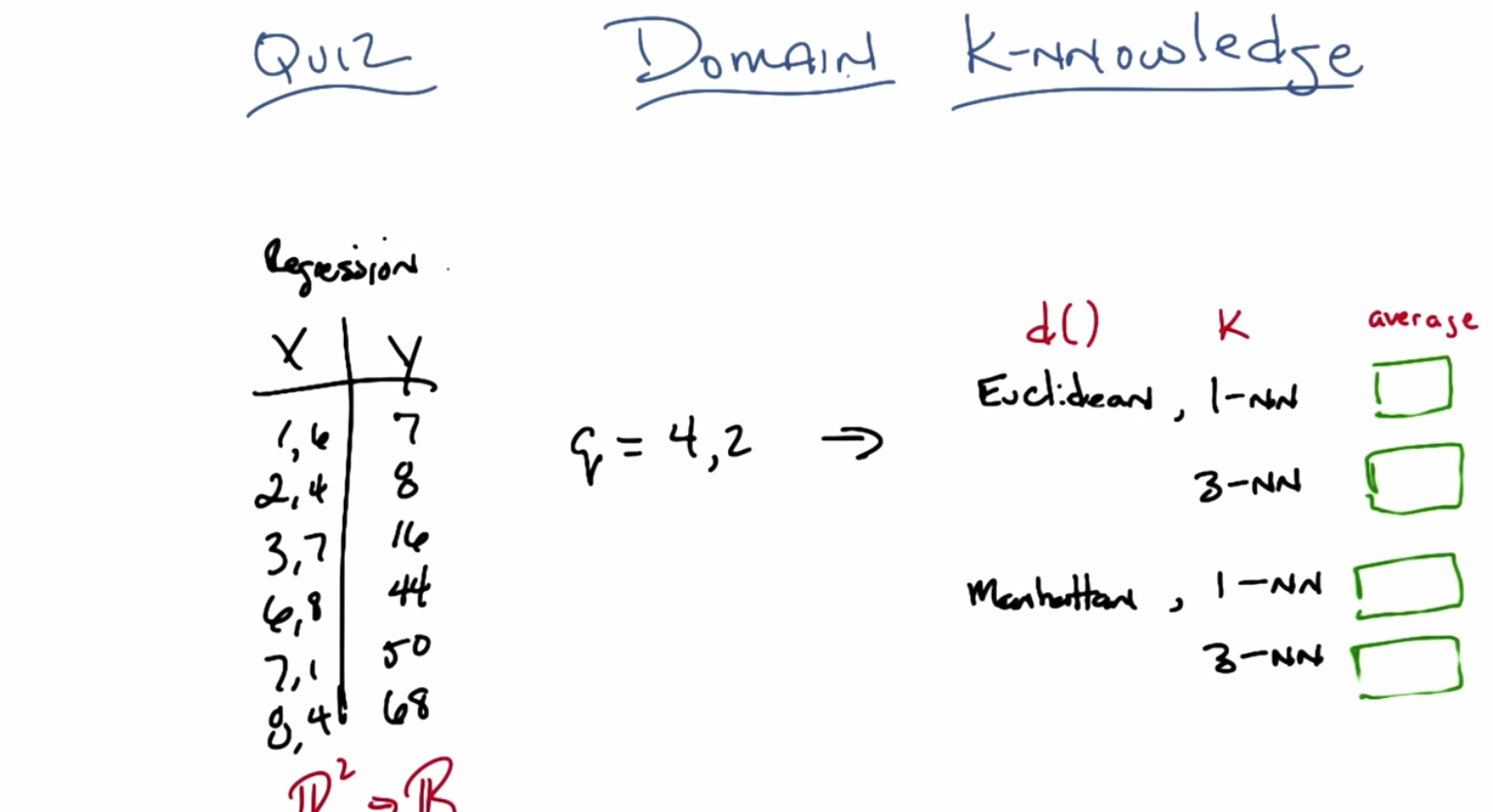
C: Okay Michael, so here’s our second quiz is a row. In the last quiz, we talked about running time and space time, but now we’re going to talk about how the k-nn algorithm, actually works. And in particular how different choices between distance metrics. Values of k, and how you’re going to put them together, can give you different answers, okay? So, what I have over here on the left is training data. This is a regression problem and you’re training data is made up of xy pairs. X is two dimensional. Okay? So this is a function from R squared to some value in R1. Okay?

M: Mm-hm.

C: The first dimension represents something and the second dimension represents something. Then there’s some particular output over here. And what I want you to do is given a query point 4, 2 produce what the proper y or output ought to be, given all of this training did. You’re with me?

M: Yeah.

C: Okay, so I want you to do it in four different cases, I want you to do it in the case where, your distance matrix is euclidean, Okay. M: The distance metric, in R2?

C: Yes.

M: Oh I see because, we’re going to measure the distance between the query and the different data points.

C: Right.

M: Yeah. Okay. Uh-huh.

C: Mm-hm. So it’s euclidean, for a case of one nearest neighbor and three nearest neighbor and I want you to take, for example, in the three nearest neighbor case. I want you take their output and average them. Okay?

M: Okay.

C: Now, in the I also want you to do the same thing. But in the case where instead of using Euclidean distance, we use Manhattan distance. But again, for both 1 nearest neighbor and we have ties, like in three nearest neighbor where we absolutely have to have at least three of these things show up, just let ‘em average. Okay?

M: Got you.

C: Now we’re doing averaging instead of straight voting because this is a regression problem.

M: Got it.

C: Okay. Any questions?

M: Maybe. Let’s see. Three nearest neighbor. And so if there’s ties we use the college ranking trick of including everybody who’s at least as good as the k, largest or k closest.

C: Yes, exactly.

M: Okay, yeah I think I can take a stab at this.

C: Okay, cool then go.

Answer

C: Alright Michael, you ready?

M: Yeah.

C: Okay. What’s the answer? Walk me through.

M: I will walk you through. Alright. So let’s do this. Let’s write the Euclidean distance. Let’s write the Manhattan distance because I don’t want to take square root to my head.

C: Okay.

M: Let’s write the Manhattan distances next to the Xs.

C: OKay.

M: Or the Ys.

C: Alright.

M: Either way.

C: Let’s do it next to the Xs. So this is the Manhattan distance or MD as the cool kids call it.

M: Is that true?

C: Yea.

M: The cool kids called it L one.

C: No, no, no have you ever heard a cool kid ever say something like L one?

M: Well, to me the cool kids are the people at neps who know more math than I do. Yea, do you think any of them are going to watch this video? Actually I’m afraid all of them are going to watch this video.

C: Now I’m really afraid.

M: Mm-Hm so you better get it right, everyone is watching.

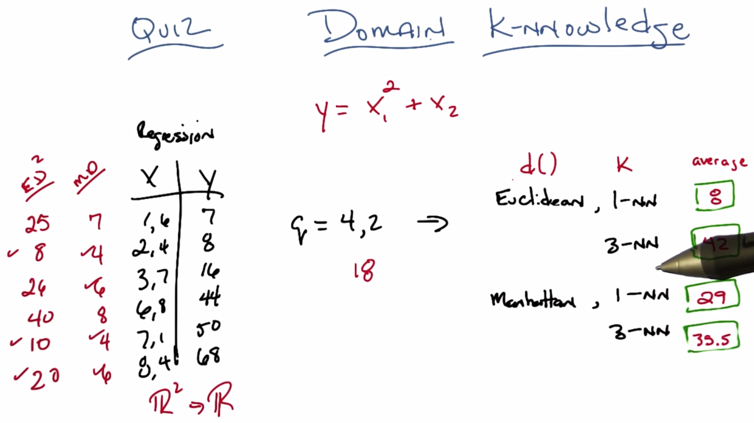
C: All right, well let me complete the Manhattan distances. So the first one what you do is you take the 1 minus 4.

M: Mm-Hm.

C: And that’s three. And you take the 6 minus 2 and that’s 4. And you add the two together and you get 7. Which interestingly is the same as y, but I think that’s a coincidence.

M: Okay.

C: And now I’ll do all the rest of them ‘cause I pre-computed them. Four, six, eight, four, six. Alright, so now we’ve got to setup so we can do one and three nearest neighbor relatively quickly. So, the one nearest neighbor, the closest distance, is four.

M: Mm–hm.

C: But unfortunately there are two points that have two comma four in set number one. We have outputs of eight

M: Uh-huh.

C: Not if we take the average of those two things we get 29.

M: Yep. That is correct Michael.

C: Great now in terms of the three nearest neighbors we have the fours and the sixes.

M: So the four, three nearest neighbors.

C: Yep.

M: Somewhat awkwardly. And we have the average of those things which Eight, fifty and sixteen and sixty eight which gets us thirty five point five.

C: Right. That was pretty straightforward. And those answers aren’t too far off from one another. So what about the Euclidean case?

M: Alright, so one thing to point out. I was worried about computing square roots but it occurs to me that I actually don’t have to compute square roots because that’s the monotonic transformation and we only care about the orders.

C: Hm, okay.

M: So for Euclidean distance, or as I like to call him casually, ED,

C: Mmhm.

M: We can just take the square differences summed up.

C: Okay, so this would be ED squared.

M: Yes, it would be ED squared.

C: Okay, ED.

M: Good. So the first one, it’ll be the one minus four is three, squared is nine.

kC: And notice the square of 25 is pretty easy to compute.

M: Yeah, but the other ones aren’t going to be. It just so happens that we’ve got a pythagorean triple on our hands.

C: Mm. I love those.

M: Al right so the remaining ones, the x squared are eight,

C: Hm, none of those are easily square rootable.

M: Exactly, though 40 feels like it really was trying and failed.

C: Yeah. An eight over shot and now it’s a perfect cube. So eight is the smallest distance.

M: Yep.

C: And coincidentally the Y value associated with that is eight.

M: Hm.

C: So an eight, eight is our answer.

M: Good and that’s correct.

C: And the three closest are eight, ten and 20.

M: Mm-hmm.

C: And if we average the Y values for those that’s eight, 50 and 68, which gives us an average of 42. The meaning of life, the universe and pretty much everything?

M: Yes! And that is absolutely correct. That’s kind of cool that you get completely different answers depending upon what you do.

C: Yeah, it does seem very different, doesn’t it? I mean there’s like several orders of magnitude spread here.

M: Well.

C: Maybe not orders of magnitude but orders of doubling.

M: Yes, there are orders of doubling spread. Well, you know what Michael, I actually had a specific function in mind when I did this.

C: Okay! Let’s find out which one is the right one!

M: Well, the function I had was Y was equal to the first dimension squared plus the second dimension. So, let’s call that X1 and X2, and this was actually the function that I had in place. So, you square the first term and you add the second.

C: Okay, and so like looking at the second last one, for example, seven squared is 49 plus one is 50. It’s very consistent.

M: Thank you. So what would be the actual answer for four comma two?

C: Okay so four squared is 16 plus two is 18. Which is close to none of them.

M: Right. So there’s a lesson here, there’s several lessons here. And one lesson I don’t want you to take away. So here’s the lesson. So I actually had a real function here. There was no noise. It was fairly well represented. The proper answer was 18 and basically none of these are right. But the first thing I want you to notice is you get completely different answers, depending upon exactly whether you do one versus three, whether you do Euclidean versus Manhattan. And that’s because these things make assumptions about your domain that might not be particularly relevant. And this sort of suggests, that maybe this thing doesn’t do very well. Cannon doesn’t do very well because none of these are close to 18. That seems a little sad. But I’ve good new for you Michael.

C: Okay.

M: The good news is that, actually cannon tends to work really, really well. Especially given it’s simplicity, it just doesn’t in this particular case. And there’s really a reason for that. It has to do with this sort of fundamental assumptions in bias of K and N, I happen to pick an example that sort of violates some of that bias. So I think it’s worth to take a moment to think about what the preference bias is for K and N and to see if that can lead us to understanding why we didn’t get anything close to 18 here.

C: Okay that sounds useful.

M: Okay, so let’s do that.

K-NN Preference Biases

scribble

slides

transcript

C: Ok, Michael, so I’m going to talk a little bit about bias. In particular, the preference bias for K. So, let me remind you what preference bias is. Preference bias is kind of our notion of why we would prefer one hypothesis over another. And they say all things, other things being equal. And what that really means is, it’s the thing that encompasses our belief. About what makes a good hypothesis. So in some of the previous examples that we used it was things like shorter trees, smoother functions, simpler functions, those sorts of things were the ways that we expressed our preferences over various hypothesis. And cannon is no exception. It also has preference by its built in as does every algorithm of any note. So I just wanted to go through three that I thought of is as being indicative of this bias. And they’re kind of all related to one another. So the first one is a notion of locality. Right? There’s this idea that near points are similar to one another. Does that make sense to you?

M: Yeah. Yeah. That was really important. It came out nicely in the the real estate example. Right. So the whole idea. The whole thing we are using to generalize from one thing to another is this notion of nearness.

C: Right. And exactly how this notion of nearness works out. Is embedded in whatever distance function we happen to be given. And so, there’s further bias that might come out, based upon exactly the way we implement distances. So, in the example we just did, euclidian distance is making a different assumption about what nearness or similarity is, compared to Manhattan distance, for example.

M: So is there like, a perfect distance function for a given problem?

C: There’s certainly a perfect distance function for any particular problem.

M: Yeah, that’s what I mean. Not one that works for the universe, but one if I give you a problem and you can work on it all day long. Can you find, is there a notion that there’’s a distance function that would capture things perfectly?

C: Well, it has to be the case for any given fixed problem. That there is some distance function that minimizes, say, some of squared errors or something like that. First is some other distance function. Right?

M: Okay.

C: That has to be the case. So there, there always to be at least one best distance function given everything else is fixed.

M: That makes sense.

C: Right. What that is who knows. Maybe you finding it might be arbitrarily difficult. Because there’s at least an infinite number of distance functions.

M: Well yeah, I was thinking that, that for latter to find distance functions to be anything we want. What about a distance function that said the distance between all the things that have the same answer is zero.

C: Mm-hm.

M: And the distance between them and the ones that have different answers is you know, infinity or something big.

C: Yeah.

M: And then, then the distance function, like, somehow already has built in the solution to the problem because it’s already put the things that have the same answers together.

C: Right, you could do that and doing that would require again solving the original problem. But yeah. So, such a function has to exist, there’s always noise. What if there’s noise in your data, you know? But some such function like that has to exist, the question is finding it. But I think the real point to take there is, there are some good distance functions for our problem and there are some bad distance functions for our problem. How you pick those is really fundamental assumption you’re making about the domain. That’s why it’s domain knowledge.

M: Yeah, that sounds right.

C: Mm ‘Kay. So, locality however it’s expressed to the distance function that is similarity. Is built in to KNN that we believe that near points are similar. Kind of by definition. That leads actually to the second preference bias which is this notion of smoothness. That we are choosing to average. And by choosing to look at points that are similar to one another. We are expecting functions to behave, smoothly. Alright, you know in the two D case. It’s kind of easy to see, right? You, have these sort of points and you’re basically saying, these two points should somehow be related to one another more than this point and this point. And that sort of assumes kind of smoothly changing behavior as you move from one neighborhood to another. Does that make sense?

M: I mean, it seems like we’re defining to be pretty similar to locality.

C: In this case. I’m drawing an example, such that whatever we meant by locality has already been kind of expressed in the graph.

M: Okay.

C: And picking this is really for pedagogical reasons. You know can imagine, this you know, these are points that live in visualize them much less draw them. And I could try. [LAUGH] But here’s three dimensions and here’s the fourth dimension. I think I’m going to get tired before I hit seven and seven thousand but, you kind of get the idea, right? If you can imagine in your head points that are really near one another in some space you kind of hope that they behave similarly. Right.

M: Right. Okay, so locality and smoothness. And I think these make sense. I mean, these, this is hardly the only algorithm that makes these kind of assumptions. But there is another assumption which is a bit more subtle I think. Which is worth spending a second talking about. For at least the distance functions we’ve looked at before, the Euclidian distance and the Manhattan distance. They all kind of looked at each of the dimensions and subtracted them and squared them or didn’t or took their absolute value and added them all together. What that means is we were treat in at least in those cases that all the features mattered. And not only did they matter they mattered equally. Right. So think about the the last quiz I gave you. Right. It said y equals x 1 squared plus x 2. And you noticed we got answers that were wildly off from what the actual answer was. Well if I know that the first dimension. The first feature is going to be squared and the second one is not going to be squared. Do you think either one of these features is more important or more important to get right?

C: Okay. Right. Trying to think about what that might mean. So, if, yea its definitely the case that when you look for similar examples in the database you want to care more about X1 because a little bit of a difference in X1 gets squared out. Right? It can lead to a very large difference in the corresponding Y value. Whereas in the x2’s, it’s not quite as crucial. If you’re off a little bit more, then you’re off a little bit more, it’s just a linear relationship. So yeah, it does seems like that first dimension needs to be a lot more important, I guess, when you’re doing the matching. Then the second one.

M: Right so, we probably would have gotten different, I’m not going to go through this but, we probably would have gotten different answers in the Euclidian or Manhattan case we had instead of just taking the difference between the first two The first dimensions, we had taken that difference and squared it. And then in the case, including this and squaring it again, and then some of those things that were closer in the first dimension instead of the second dimension would’ve looked more similar and we might’ve gotten better answer. That’s probably a good exercise to go back and do for someone else.

C: [LAUGH] Yeah, I was thinking of doing it right now. But yeah, probably should leave it for other people.

M: Well you can do it if you want to. So did you do it Michael?

C: I did.

M: And?

C: So it’s a kind of now a mix between the Manhattan distance and the Euclidian distance. So, I’m taking the first component, take the difference, square it.

M: Mm-hm.

C: Take the second component, take the difference, absolute value it. And add those two things together.

M: Sure.

C: All right. So if I do that, with one nearest neighbor, I still get that tie, but the output answer ends up being 12.

M: Hm. Which is better than 24.7.

C: And that’s better than eight, which is what it was before. So the eight has gone up to think was 35.5, comes down to 29.5 Close here again to the correct answer which is eighteen. So in both cases it kind of pushed in the right direction. The answers that were relevant and fewer of the answers that were not relevant.

M: Right. There you go. So the notion of relevance by the way, turns out to be very important. And highlights a weakness of Knn. So this brings me to a kind of theorem or fundamental results of a machine learning that is particularly relevant to Knn but its actually relevant everywhere. Do you think its worth while to mention it?

C: Sure it sounds relevant.

M: Alright let’s do it.

Curse of Dimensionality

scribble

slides

transcript

C: Okay, Michael. So this notion of having different features or different dimensions throw us off has a name and it’s called the Curse of Dimensionality.

M: Oh, nice audio effect.

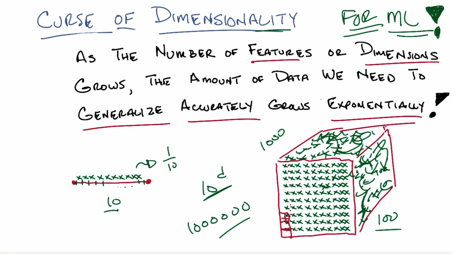
C: I did like that effect in post-production. And it refers to well, a very particular thing. So let me just read out what it refers to. As the number of features or equivalently dimensions grows that is as we add more and more features we go x of 1, x of two then we add x of three, add more and more of these features. As those features grows or as the number of dimensions grow ,the amount of data ,that we need to generalize accurately also grows exponentially. Now this is a problem of course because Exponentially means, bad in computer science land because when things are exponential they’re effectively untenable. You just can’t win.

M: I think everybody knows that in the sense that if you look, I’ve done this experiment actually, if you look in the popular press like, you know, Time Magazine Or New York Times, USA Today. People will use the word exponentially sometimes to mean exponentially, and sometimes to mean, a lot.

C: Yeah that’s actually a pet peeve of mine. The whole notion.

M: Me too.

C: Oh, it’s exponentially bigger. No, that’s, that’s not meaningful. If you’re saying I have one point. And then I have another point, and I want to say this one point is exponentially bigger than this one. That’s meaningless! It’s also literally bigger than that one. Exponentially refers to a trend.

M: Again, they’re not talking about the mathematical relationship. They just mean a lot.

C: Okay, so they’re wrong. And it bothers me deeply but I’m willing to accept it for the purposes of this discussion. Okay. Exponentially means bad. It means that we need more, and more data as we add features and dimensions. Now as a machine learning person this is a real problem because what you want to do, or like what your instinct tells you to do is, we’ve got this problem, we’ve got a bunch of data, we’re not sure what’s important. So why don’t we just keep adding more and more and more features. You know, we’ve got all these sensors and we’ll just add this little bit and this little bit, and we’ll keep track of GPS location and we’ll see the time of the day and we’ll just keep adding stuff and then we’ll figure out which ones are important. But the curse of dimensionality says that every time you add another one of these features. You add another dimension, to your input space, you’re going to need exponentially more data, as you add those features, in order to be able to generalize accurately. This is a very serious problem, and it sort of captures, a little bit of what the difficulties are in k and n. If you have a di, if you have distance function or a similarity function, that assumes that everything is Relevant, or equally relevant, or important, and some of them aren’t. You’re going to have to see a lot of data before you can figure that out, sort of before it washes itself away.

M: Yeah, that makes a lot of sense.

C: Yeah, it seems a little scary. So, you know, I think you can say these words, and the words sort of make sense, but I think it helps to kind of draw a picture, and so I’m going to draw a little picture. Okay?

M: Yeah.

C: All right.

Curse of Dimensionality Two

scribble

slides

transcript

C: Okay, Michael, so let’s, let’s look at this little line segment, okay? And then say I’ve got ten little points that I could put down on this line segment, and I want them all to represent some part of this line, alright? That’s kind of KNN nearest neighborish. So, I’m going to put a little X here, I’ll put one here, I’ll put one here, put one here, put one here, here, here, here, here, here. Is that ten? Three… six. Nine, ten. Ten. Okay. And let’s pretend I did the right thing here and I have them kind of uniformly distributed across the line segment. So that means each one of these points is sort of owning, an equal size sub segment of this segment. Does that make sense?

M: Yeah, so it’s representing it in the sense that point. Uh, when you’re trying to estimate values of other places on the line it’s going to default as the nearest neighbor to being that point so there’s a very small little neighborhood of the red line segment that is covered by each of the green X’s.

C: That is exactly right and in fact each one of these green X’s represents. How much of this segment?

M: Each of the green X’s covers one tenth?

C: That’s exactly right. You cover one tenth. Alright Michael, so let’s say I move from a line segment now to a two dimensional space. So a little square segment. If that’s the right technical term. And I’ve taken my little ten x’s, and I put them down here before. Well, here’s something you’ll notice; you’ll notice that each one of these x’s is going to still end up representing onetenth of all of this space, but you’ll also notice that, that, that it’s representing now you know. Really really really really big.

M: I see.

C: So one way of putting it is, you know if you think about the farthest point, as opposed to the furthest point which would be incorrect. The farthest point that this particular first x over here is representing, its got some distance here. Over here, the farthest point from this x, the distance is very far away. So, a question would be, how can I make it so that each of the x’s I put down represents the same amount I don’t know diameter or distance as the xs in this line segment over here? So what do you think I have to do?

M: I feel like you need to fill up the square with xs.

C: Yeah, that’s exactly right so let’s do that. So filling em up Michael as you suggested. You’ll notice that at least if we pretend that I drew this right. Each of these X’s is now going to end up being the nearest neighbor for a little square like this, and the diameter of these little squares are going to be the same as the diameter of these little line segments.

M: Yeah, I agree for some definition of the word diameter.

C: Yes, and for some definition of our demonstration. Okay, so how many of these X’s are there, Michael? Can you tell? You want to count?

M: I’m going to multiple cause it looks like you did ten by ten so that’ll be 100.

C: That’ll be 100. So each one now holds a hundredth of the space, and I went from needing ten points to, of course, 100 points in order to cover the same amount of space.

M: Alright, so that definitely seems like the mild rebuke of dimensionality.

C: Yes.

M: But doesn’t seem that bad.

C: Okay well, what happens if I now move into three dimensions? So now, if I want to cover the same amount of, you know, diameter space for, you know, sufficient definition of diameter. I’m going to have to do a bunch of copying and pasting that I’m not willing to do so, you know, there would be more x’s here and you know, there will be x’s there and an x here and it’ll just kind of go and fill up some space and you know, I’m not going to do this whatever but [SOUND] and you’ll get x’s everywhere. And you notice, I need a lot more X’s than I had before. And by the way, I’m just showing you the outside of this little cube, there are actually X’s on the inside as well, that you can’t see. How many X’s do you think I have?

M: I don’t think you drew any X’s. You’re just like scribbling on the side of the cube.

C: These are X’s.

M: You, you were doing so well for awhile, and then just lost it entirely.

C: Well, wouldn’t you lose it if you had to write 1000 x’s.

M: Hm. No because I would use computers to help me but yes, yes it is very frustrating to have to have that many x’s. And so but in particular in this case we’re talking about data points in a nearest neighbor method and boy that does seem like a big growth from ten to a 100 to 1000.

C: In fact the growth is exponential.

M: Exponential.

C: Right. So if we went into four dimensions, which I’m not going to draw, then we would need need 10,000 points. And in six dimensions, we would need 1,000,000 points. And so on and so forth. So something like. Ten to the D, where D is the number of dimensions.

M: Wow.

C: Right. So this is really problematic right. In my little nearest neighbor method, I want to make sure the neighborhood remains small as I add dimensions, I’m going to need to grow the number of points that I have in my training set exponentially. And that’s really bad. And by the way, this isn’t just an issue Of k-nn. This is true in general. Don’t think about this now as nearest neighbors in the sense of of knn. But think of it as points that are representing or covering the space. And if you want to represent the same sort of hyper-volume of space as you add dimensions, you’re going to have to get exponentially more points in order to do that. And coverage is necessary to do learning. So the curse of dimensionality does not just to K and N. It is a curse of dimensionality for ML period.

M: You mean for me?

C: Yes.

M: Okay. And that seems really problematic because it’s very natural to just keep throwing dimensions into a machine learning problem. Like it’s having trouble learning. Let me give it a few more dimensions to give it hints. But really what you’re doing is just giving it a larger and larger volume to fill.

C: Yeah. And it can’t fill it unless you give it more and more data. So you’re better off giving more data than you are giving more dimensions.

M: Zoinks.

C: Mm-hm. There’s an entire series of lessons that we will get eventually that, that deals with this issue.

M: The issue of?

C: Dimensionality.

M: Finding the right dimensionality?

C: Yeah.

M: That would be a useful thing.

C: It would. But it’s far off in the future. It’s like infinitely far in the future. So we’ll worry about that in a few weeks.

M: Okay.

C: Okay. All right. So there you go, Michael. Curse of Dimensionality is a real problem.

M: Where did that term come from, it’s a cool term. I think it came from, oh what’s his name. Bellman.

C: Oh, Bellman, like the dynamic programming guy.

M: Yeah, the dynamic programming guy, the Bellman of Bellman equation guy.

C: Which we haven’t gotten to that yet in the course.

M: Which we haven’t gotten to in the course but we will get to in the course. Because it’s central. So it looks like the element’s central to a lot of things.

C: Wow.

M: Sometimes it gives us equations that helps us but sometimes it gives us curses.

Some other stuff

scribble

• locally weighted linear regression.
• The notion of replacing average with regression or some other classification function helps us to do more than we could think.

slides

transcripts

C: Okay, Michael so we talked a little bit about the curse of dimensionality, but I think it’s worthwhile to talk about some other stuff that comes up. We’ve been sort of skirting around this and you know bring it up in various ways throughout our discussion so far. But I think it’s worthwhile kind of writing them all down on a slide and trying to think through them for a little bit. So the other stuff that comes up in knn mainly comes up in these sort of assumptions we make about parameters to the algorithm. So the one we talked about the probably the most is our distance measure, you know our distance between some X and some query point Q and we’ve explored a couple. We looked at Eucudean and we looked at Manhattan. And we even looked at weighted versions of those. And this really matters, I’ve said this before but I really think it bears repeating that your choice of distance function really matters. If you pick the wrong kind of distance function, you’re just going to get very poor behavior.

M: So I have a question about these these distance functions. So you mentioned Euclidean and Manhattan, are there other distance functions that the students should know? Like, things that they, that might come up, or things that they should think of first if they have a particular kind of data?

C: yeah, there’s a, there’s a ton of them. I think Well, first off, it, it’s probably worth pointing out that this, this notion of weighted distance is one way to deal with the curse of dimensionality. You can weigh different dimensions differently. And that would be one and you might come up with sort of automatic ways of doing that. That, that’s sort of worth mentioning. But you will notice that both Euclidean and Manhattan distance at least as we have talked about them, are really useful for things like regression. Their kind of assuming that you have numbers in that subtraction kind of makes sense. But there are other functions, distance functions that you might do if you are dealing with cases like, I don’t know Discrete data, right? Where instead of it all being numbers, it’s colors, or something like that. Alright so, your distance might be mismatches. For example, or it might be a mixture of those. In fact, one of the nice things about KNN, is that we’ve been talking about it with points because it’s sort of easy to think about it that way. But this distance function is just a black box. You can take Arbitrary things and try to decide how similar they are based on whatever you know about the domain and that could be very useful. So ,you could talk about images right. Where you take pictures of people and you know rather than doing something like a pixel by pixel comparison, you try to line up their eyes. And look at their mouths, and try to see if they’re the same shape you know things like that, that might be more complicated and and perhaps even arbitrarily computational to determine notions of similarity so really this idea of distance in similarity tells you a lot about your domain and what you believe about it. Another thing what’s pushing on a little bit is how you pick k. Well there’s no good was to pick k. You just have to know something about it, but I want to think about a particular case. Well, what if we end up in a world where K=N. C: Well, that would be silly.

M: Why would it be silly?

C: So if K=N, then what you’re doing is you’re taking in the case of regression for example, you’re taking all of the data points and averaging the y values together. Basically ignoring the query. So, you end up with a constant function.

M: But that’s only if you do a simple average. What if you do a weighted average?

C: A weighted average. So the near, the points that are the query are going to get more weight in the average, so that actually will be different. Even though k equals n, it will be different depending on where you actually put your query down.

M: Exactly. That’s exactly right so, for example, if I have a little bunch of points like this say. Where you notice it kind of looks like I have two different lines here and I pick a query point way over here. All of these points are going to influence me as oppose to these points and so I’m going to end up estimating with something that looks more like this because these points over here won’t have much to say. But if I have a query point that’s way over here somewhere these points are going to matter and I’m going to end up looking something looks a little bit more like this than that. Now I’m drawing these as lines. They won’t exactly look like lines because these points will have some influence. They’ll be more curvy than that. But the point is that near the place we want to do the query it will look to be more strongly influenced by these points over here or these points over here depending on where you are.

C: Well that gives me an idea.

M: Oh, what kind of idea does it give you?

C: Well, what about instead of just taking a weighted average, what about using a distance matrix to pick up some of the points? And then do a different regression on that substantive point.

M: Right, I like that. So we can replace this whole notion of average with a more kind of, regression-y thing.

C: So instead of using the same value for the whole patch. It still continues to use the input values.

M: Yeah. So in fact, average is just a special case of a kind of regression, right?

C: Mm hm, mm hm.

M: Right? So this actually has a name, believe it or not. It’s actually called locally weighted regression. Yeah, so this actually works pretty well and in place of sort of averaging function, you can do just about anything you want to. You could throw in a decision tree, you could throw in a neural network, you could throw in lines do linear regression. You can do, almost anything that you can imagine doing.

M: Neat

C: Yeah. Add that works out very well. And again, it gives you a little bit of power. So here’s something I don’t think is very obvious until it’s pointed out to you. Which is this notion of replacing the average with a more general regression or even classification function. It actually allows you to do something more powerful than it seems. So let’s imagine that we were going to do locally weighted regression and we were going to do linear regression. So, what would locally-weighted linear regression look like? Well, if we go back to this example over here on the left basically, you take all the points that are nearby and you try to fit a line to it. So you would end up with stuff that looked like this. While you’re over here, you would get the line like this, but while you were over here you’d get a line like this. Then, somewhere in the middle you would get lines that started to look like this and And you would end up with something that kind of ended up looking a lot like a curve. So that’s kind of cool because you notice that we start with a hypothesis state of lines and this locally weighted linear regression. But then we end up actually being able to represent a hypothesis space that is strictly bigger. Then the set of lines. So we can use a very simple kind of hypothesis space but by using this locally weighted regression we end up with a more complicated space that is complicated, that’s made more complicated depending upon the complications that are represented by your data points. So this results, this sort of reveals another bit of power with k-nn. Which is, it allows you to take local information and build functions or build concepts around the local things that are similar to you. And that allows you to make arbitrarily complicated functions.

M: Neat.

Summary of Instance Based Learning