Kernel Methods and SVM

scribble

• Least commitment line in multiple dimensions.

slides

transcript

C: Ok, so today we’re going to talk about support vector machines and I’m going to do something unexpected. I’m going to start out the beginning of this with a quiz.

M: With a quiz.

C: Yes, with a quiz. So here’s the quiz for you, Michael. I’ve drawn some points labeled positive and some labeled minus, representing two different classes. And, you’ll notice that you can draw a line to separate them, therefore they are…

M: Linearly separable.

C: Exactly. So the question I have for you is simply this, which is the best line? And here’s how you’re going to show me. Here’s how you’re going to show me. I’m not just going to ask you to draw some random line because that’s too hard for us to get feedback on. So instead what I’ve done is I’ve drawn three green dots. Here on the sort of upper left and three red dots here on the bottom right and what I want to you to do is select one of the green dots and one of the red dots and since you’ll have two dots that will define a line and that’ll be the way you indicate to me which of the lines is in fact the best line.

M: The best line.

C: The best line. And I’m not going to even tell you what best means. You tell me what best means, when you justify why you would choose one over the other.

M: If I think they’re all the best, I can choose any one I want?

C: That’s right. Ok. So you got it?

M: I think so.

C: OK. Go.

Answer

C: Alright, Michael. So, you got it? Which line do you think is best?

M: Alright, so if I choose one green and one red that means there’s nine different possible lines. But they all separate the points.

C: That is correct.

M: So, I mean the only one that seems special is the middle one. If I choose the middle green and the middle red it’s kind of, you know, aesthetically pleasing. There’s a lot of space on each side. So, I’m going to go with that.

M: Yes.

C: And you think that’s best. Well, I’m going to give you a hint, Michael, and tell you that you were correct. That’s a pretty good hint.

M: Yeah.

C: But now I want you to figure out for me why that line is better than this line.

M: Interesting. So one thing that the second line has against it is that it seems to get really, really close to that bottom minus point. Maybe it’s a little too close. Like maybe that minus is near other minuses that we just can’t see. And since we drew it really close, it could be we ended up chopping of some of the minuses that we might want to have kept on the other side. And so maybe by drawing it in the middle it’s sort of, we have the biggest demilitarized zone.

C: No, I like that. So that is a very good explanation for why you would prefer the middle line over the other line that isn’t the middle line. And you can make a similar argument for any other of the nine lines that you could possibly draw. Let me draw another line for you and you tell me if you think this one is good or bad and why it might be better or worse than the middle one. See if you give me a different answer. I can take one of the parallel lines which again we will pretend is a straight line and put it there. Or I can take in fact the other line that is meant to be parallel to it and why aren’t those lines better? Or just as good.

M: I guess I’d use the same explanation as before which is that these, the, the line that was, is really close to the pluses maybe is a little too close for comfort and it, it gets very close to that plus. The, kind of, I don’t know. I could point to it, but maybe you should point to it. The plus that’s really close to the line.

C: I’m pointing to it.

M: Because again if there’s just, you know, other data points near there, it’s going to make this distinction between the positives and the negatives that isn’t really warranted by the data.

C: Right, so I could make the opposite argument with you, Michael, which is that listen, they all separate the points. They completely explain the data as we see them. So, all three of those lines explain the data. In fact, all nine of those lines explain the data. So, why aren’t they warranted by the data? What’s the problem that you might run into if you put one line very close to the positives or one line very close to the minuses?

M: Well, again…so, so…it may be that they fit this data. But, this is just a sample from the population. And so… you know, we don’t know what’s going to happen really close to that other plus is. So like in the nearest neighbor algorithm for example which you always try to make me remember, it’s going to want to, you know, if it’s closer to the pluses, it should be a plus.

C: Right. That makes sense and I think that’s exactly right so your intuition and I think the intuition that people should take with them is that lines that are too close to the positives. Or lines that are too close to the negatives, sort of have this feature where you’re believing the training data that you’ve got too much. You’ve decided that all of these boundaries are fine because of the specific set of training data that we’ve got. And while you want to believe the data, because that’s all you’ve got, you don’t want to believe the data too much.

M: That’s overfitting.

C: That’s overfitting. So, the problem with those two lines, or one way to think about the problem with those two lines, is that these lines are more likely to overfit. And why is that? It’s because they’re believing the data too much. So, given that we’re trying to avoid overfitting, what could you say about the middle line? So, here’s the argument that I would make, and you tell me if you buy it, Michael. This line, or the line it’s intended to represent anyway, is the line that is consistent with the data while committing least to it. That seems like a good way of saying what I was feeling, yeah. It is funny though because like, overfitting up to this point, we you, we were generally talking about overfitting as being something where there’s a great deal of model complexity in some sense.

M: And it doesn’t seem like those lines that are closer to the pluses or closer to the minuses. Are inherently more complex, they’re still lines. It’s interesting that they, they, they kind of maybe behave as if they are.

C: Right, and in fact they, they’re, it’s a more, sort of, literal interpretation of the words over and fit, right? You, you have decided to fit the data, and you believe it too much, and what you really want to do is commit. The least that you can commit to the data while still being consistent with it right. So this basic idea of, uh,uh, finding the line of least commitment in the linear separable set of data, is the basis behind support vector machines. So what I want to do next is I want to see if we can come up with some equation that would help us define such a line. It’s easy in this case cause we’re staring at it but if you imagine these points were in plane just by staring at it so let’s see if we can try to work out how you go about finding this least commitment line.

Support Vector Machine

scribble

slides

transcript

C: Okay Michael. So, let’s write down a few equations. Let’s try to be a little bit more formal. A little bit more mathematical about this idea. So, I’m going to try to encapsulate, what we just talked about, the line of least commitment, by drawing another line. So, if we think of this top gray line here as sort of the line that gets as close to the plus points as possible, without crossing over them and mis-classifying them, and we think of the bottom gray line as the one that gets as close as possible to the minus signs without crossing over them and misclassifying them, and then the middle line is sort of in the happy medium. Okay? So, what you really want is that, somehow, this distance between these lines is as big as possible. Can you see that?

M: Yeah, though it seems like the gray line could be pushed out a little more, right? The minuses don’t bump into it.

C: That’s a good point Michael and I’m going to fix that by putting a minus sign here.

M: Okay

C: I did the best I could under the circumstances.

M: Data, revisionist history.

C: No, there’s just an invisible point, and I just made it more visible. For the sake of the reader. Okay, so, I’ve got these two lines, these are sort of as far as I can go without starting to do mis-classification with my separating line, and the line in the middle, we’ve already argued, is the sort of the best one because it provides the least commitment. So, that means you want to have a line that leaves as much space as possible from the boundaries. Alright, Michael. So let’s see if we can figure out exactly what that line is like. So, the first thing, that I want to do is, is introduce a little bit of notation. Right? So we all remember what the equation, of a line is. It’s , that’s just a general equation for a line. But, here even though we’re going to be drawing with lines, we really want to deal with the general case, where we’re talking about hyperplanes. And generally ,when we write about hyperplanes, we describe them as some output, let’s just call it . Here, because of what we’re trying to do with classification, the output y is going to be some value that indicates whether you’re in the positive class or you’re in the negative class. W represents the parameters for our plane along with b, which is what moves it out of the origin. Okay, are you with me?

M: I think so, but that’s, so maybe we should get rid of that top y because that y is different kind of y. The top y is talking about the y dimension of the plane and in the second equation, that y is kind of folded into the x. And we have a new y, which is actually, the output of the classifier.

C: Right. I like it, so let’s get rid of that first y which is just an equation for a line and let’s ask what each of these things are. So, let’s just say that again for clarity’s sake. I think, you make a good point, Michael. Y here is going to be our classification label whenever we’re talking about using a linear separator. What we’ve been talking about, which I realize now we never ever actually said explicitly, is that you are taking some new point, projecting it onto the line, and then looking at the value that comes out from projecting it. And in this case, in particular, we want positive values to mean yes, you are part of the class, and negative values to mean that you aren’t a part of the class. Okay?

M: Yep.

C: This is our classification label y. W represents again, the parameters of the plane along with b, which is what moves it in and out of the origin. So, this is now, effectively, what our linear classifiers actually look like. Even in multiple dimensions with hyperplanes. Okay? Cool. So, let’s take that and and push it to the next level. Let’s figure out exactly what we would expect the output of our hyperplane to be in this example that I’ve drawn on the screen here. So, we know we want to find this orange line in the middle, which has the property that it is your decision value. It tells you whether you are in the positive class or negative class, on the one hand, but also, it has the property of being as far away from the data as possible while still being consistent with it. So, if you’re on the decision boundary for this particular line, which again, is , what would be the output of this classifier for any point that lies along the line?

M: So, right, if that’s the decision boundary, that’s where it’s kind of not sure if it’s positive or negative, so that should be zero.

C: Right, so the equation of this line or this hyperplane, is for some set of parameters W and b. Since it’s at the decision boundary, it should give me neither a positive or a negative output. Okay?

M: Yep.

C: Okay now, one question we can ask ourselves then, if we look at these other lines is, what’s the equation for the other gray lines that are right at our positive or negative examples? So to help you answer that, I want to talk about what the labels themselves ought to be. So, just like we did with boosting, let’s say that our labels are always going to be from the set {-1, +1}. We know that our labels are -1 and +1, so we’re going to take advantage of that fact by saying that the line that brushes up against the positive example should output +1 on the very first point that it encounters. Does that make sense?

M: Yeah

C: Okay

M: That way the things that are kind of past the line are going to be +1 and the things before the line in kind of that demilitarized zone are going to be between zero and +1.

C: Right, so in fact given what you just said, what is the equation of that line?

M: Oh I see. So, it should be .

C: That’s exactly right. And by a similar argument, where would you say the, the line of the hyperplane should be for the bottom gray line? Analogously, it seems like that one should be . M: Right. So we have the decision boundary and we know that the equation of the line is . We know that if we slid that line towards the positive values, we would end up with . And if we slid it towards the negative values, we’d end up with . Now we can ask ourselves, how does this helps us? And it helps us in a very a simple way. We know that we want the boundary condition line, the one that is actually our decision boundary, to be as far as possible from both the positive and negative examples, so that would mean then that the distance between the two gray lines, which are parallel to that line, needs to also be maximized.

C: Yeah, that’s exactly what we want.

M: Right, so we want this vector here to have the maximum length that we can have. Okay, so, how are we going to figure out how long that particular line is? So, here is a simple idea. Well, the lines are parallel to one another. We can pick points on that line to define that particular distance there. So, just because it’s really easy to do the math, I’m going to chose a point here and a point here. Those points have the property, that, if I draw the line between them, you get a line that is perpendicular to the two gray lines. And I don’t know what their respective x values are, so I’m just going to call, them x1 and x2, and that is going to define the two points that I have. The vector that is defined by their difference is in fact going to have the length that tells you how far apart those two lines are, which, in turn, because of the way that we’ve constructed them, tells you how far apart your boundary decision line is from the data and we want that to be maximized because then we made the least commitment to the data. So, let’s write that down as algebra. The equation for our positive line is . And all I’ve done there is substitute, some point – I don’t have to know what is, it’s going to turn out – that puts me in some particular place on that line. And similarly, I can do the same thing for my negative line and get . Now, we want the distance between these two hyperplanes (or lines in this example) to be maximized. In order to figure out what that means, we need to know exactly what that line is. So it’s the difference between the two. So, we can just use our favorite trick when we’re doing systems of linear equations and just subtract the two lines. We basically have two equations and two unknowns. And, we simply subtract them from one another so that we can get a single equation that happens to represent the distance between them. So, if I subtract the two from one another, what do I get?

M: A quiz.

C: Oh, I like that, we get a quiz. That is the correct answer.

Quiz: Distance Between Planes

scribble

• Maximize the margin.

slides

transcript

C: Okay. So here’s the quiz. Michael is going to answer it, but we want to give you a chance to answer it first. I’ve got these two equations of two different hyperplanes, though they’re parallel to one another because they have the same parameters. That is to say, I have two equations and two unknowns. I want to subtract them from one another and what we want you to do is we want you to solve for the line that is described by their difference. Do you understand that, Michael?

M: Yeah, I think I’m just going to subtract the second equation from the first equation. It seems pretty straightforward.

C: Okay, it seems reasonable to me. But remember, the output that I want you to figure out here is exactly what the distances between those two planes, okay? That is, between what’s represented by x1 and x2, okay? Go.

Answer

C: Okay Michael, what’s the answer?

M: Well, there’s the answer to the question that I thought you were asking and then there’s the question that you then, at the end, actually asked. It seems like at the end you asked what is the distance between the two lines and I feel that that’s just the norm of x1 minus x2. But the difference between these equations is going to be well, …

C: Well why not write down what you’re telling me over on the side over here and then we can put the final answer in the box.

M: Okay.

C: Okay, so what now?

M:

\[w^T ( x_1 - x_2 ) = 2\]

C: Right, so you used the power of subtraction to make that work. Okay, very good. Okay, so that’s the difference between those two equations, now how am I going to go from there to figuring out the distance between x1 and x2?

M: I still feel like it’s just that norm of x1 minus x2.

C: Okay, but I want you to tell it to me in terms of W because the only things we have to play with here are W and b. That’s what defines our line and I want to find the right line, so I’d like to know something about the relationship between W and the distance between x1 and x2.

M: Well, times their difference is 2.

C: [LAUGH] That’s true.

M: That’s not telling us the distance, though. So what is the distance in terms of W?

C: Well what if I told you W was a number? What would you do if it was just a simple scalar and you had this equation, and I wanted to know what x1 minus x2 was. What would you do?

M: And I wanted it in terms of W?

C: Yeah, I wanted to know what x1 minus x2 was equal to.

M: Oh, I see. So, if I divide it by W, that would be helpful because then x1 minus x2 would be \(2 / W\)

C: Right, but you can’t do that because W is a vector, and you can’t really divide by a vector, at least not in the world that we’re talking about. So how are you going to make that work? Would you like a hint?

M: Sure.

C: Well here’s a hint, we want to move w over from one side to the other. We could start doing all kinds of tricks with inverses, and with the inverse of a vector. There’s all kinds of things that you could do, but actually the easiest thing way of doing it is getting rid of W on one side. And the easiest way to do that is to divide both sides by the length of W. So, rather than dividing both sides by W, we divide them by the length of W. Now what is dividing W by the length of W?

M: So, right. So W divided by the length of W, is a normalized version of W. So it’s like something that points in the same direction as W, but sits on the unit sphere.

C: Right. No, that’s exactly right! Alright, in fact it’s a hypersphere, I suppose. So we do that and that effectively is like giving you a value 1 because, like you said, it’s a unit sphere. And so now we’re actually talking about the difference between the vector x1 and the vector x2 projected onto the unit sphere and that’s equal to .

\[\frac {w^T} {|w|} ( x_1 - x_2 ) = \frac {2} {|w|}\]

C: [LAUGH] So does that help you?

M: Does that actually answer the question? Doesn’t seem like it does.

C: No, it does.

M: So x1 minus x2, dotted with W. So W, W, we don’t know. It could be anything. Can it? So.

C: Mm-hm.

M: We’ve taken x1 minus x2 and projected it onto W. So it’s like the length of x1 minus x2, but in the W direction.

C: Exactly. So, what we’ve just done is we have found the length of x1 and x2 in the W direction. What do we know about W with relationship to the line?

M: W is the parameter to the line.

C: Yes, but in particular, W actually represents a vector that’s perpendicular to the line.

M: And since we chose x1 and x2, their distance or the difference between them would in fact be perpendicular to the line. What we’ve just done is projected the difference between those two vectors onto something that is also perpendicular to the line. And so what that ends up giving us is, in fact, its length. So we maximize the length of x1 minus x2 by doing what with W?

C: Have we answered the quiz yet by the way, or are we still working on that?

M: I’m going to say we are still working on it.

C: Alright, this is a hard quiz. The thing on left, not just where the braces are, that actually turns out to be the distance between the two. Hyperplanes.

M: Right, let’s let’s give that a letter. Let’s call it m.

C: Mm.

M: Mm.

C: And, we’re saying that equals 2 over the norm of W. And that’s, so, if we want to maximize that the only thing that we have to play with is W and that is made larger and larger as W gets smaller and smaller, in other words, pushing it toward the origin.

M: Right.

C: So it set Ws to all zeroes, and we should be golden.

M: Right, except if we push all the Ws to zero, we might not be able to correctly classify our points but what this does tell us is that we have a way of thinking about the distance of this vector and where the decision boundary ought to be. We want to find the parameters of the hyperplane such that we maximize this distance over here represented by this equation while still being consistent with the data, which makes sense because that’s actually what we said in the first place. By the way, this thing has a name and it’s the reason why I chose m – it’s called the margin, and what all of this exercise tells you is that your goal is to find a decision boundary that maximizes the margin, subject to the constraint that you actually want to correctly classify everything, and that is represented by that term. Now somehow, it feels like having gone through all this we ought to be able to use it for something and turn it into some other problem we might be able to solve so that we can actually find the best line. And it turns out we can do that.

C: Have we answered the quiz yet?

M: Oh yeah we did. Which is in fact what I wanted.

C: Wow. Somebody gets that, that would be pretty impressive.

M: That would be very impressive. Or anything similar to this I would accept. In fact I probably better will. Okay good. So, it turns out that this whole notion of thinking about finding the optimal decision boundary is the same as finding a line that maximizes the margin. And we can take what we’ve just learned, where we’ve decided the goal is to maximize and turn it into a problem where we can solve this directly.

Still Support Vector Machines

scribble

slides

transcript

C: Okay. So, we’re still talking about support vector machines, although I haven’t told you what support vector machines are yet, we’re getting there, Michael. Bear with me. And what we got from our last discussion is that what we want to do somehow is maximize a particular equation, that is, \(\frac {2} {|W|}\) And as a reminder, W are the parameters of our hyperplane. So somehow, we want to maximize that equation, subject to the constraints that we still classify everything correctly. Okay, so we want to maximize while classifying everything correctly. But, while classifying everything correctly is not a very mathematically satisfying expression, it turns out we can turn that into a mathematically satisfying expression. And let me show you how to do that. So here’s a simple equation. While classifying everything correctly turns out to be the same as, and I’m just going to write, I’m going to write it out for you, Michael, and see if you can, you can guess why this works. So, what I’ve written here is. That is, for all of our training data examples. So why does this work?

M: Well, what we really want is that the classifier, is greater than or equal to 1 for the positive examples and less than or equal to -1 for the negative examples. But you cleverly multiply it by the label on the left-hand side, which does exactly that. If yi is 1, it leaves it untouched. And if yi is negative, it makes it less than or equal to minus 1. That’s, that’s very clever.

C: It is very clever, and I’m going to pretend that I came up with that idea myself. So, it turns out that trying to solve this particular problem, maximizing , while satisfying that constraint, is a little painful to do. But we can solve an equivalent problem, which turns out to be much easier to do, and that is this problem. That is, rather than trying to maximize , we can instead try to minimize that those will always have the same answer?

M: Yes, so, well, not the same answer, but it will be a minimum. The point that maximizes one will minimize the other because we took the reciprocal. As long as we’re talking about positive things. And since these are lengths, they’ll be positive. Taking the reciprocal exactly, you know, changes the direction, of what the answer is. And the squaring is, is, makes it monotone. It doesn’t, it doesn’t, it magnifies it but it doesn’t change the ordering of things. So yeah. That, that, that seems fine. I don’t why that’s any easier, but it seems the same.

C: Well, do you want to know why it’s easier? Cause I’ll tell you.

M: Please.

C: This is easier because when you have an optimization problem of this form, something like minimizing a W squared, subject to a bunch of constraints, that is called a quadratic programming problem. And people know how to solve quadratic programming problems in relatively straightforward ways.

M: Awesome.

C: Now, what else is nice about that is a couple of things. One is, it turns out that these always have a solution, and in fact, always have a unique solution. Now, I am not going to tell you how to solve quadratic programming problems because I don’t know how to do it other than to call it up in MATLAB. But there’s a whole set of classes out there, where they teach you how to do quadratic programming. We could take an aside, I could learn all about quadratic programming, and then we could talk about it for two hours. But it’s really beside the point. The important thing is that we have defined a specific optimization problem and that there are known techniques that come from linear algebra that tell us how to solve them. And we can just plug and play and go. Okay?

M: Okay, fair enough.

C: Okay, fair enough. So, in particular, it turns out that we can transform, again, this particular quadratic programming problem into a different quadratic programming problem. Or actually, truthfully, into the normal form for a quadratic programming problem, that has the following form. So here’s what this equation tells you, Michael. We have basically started out by trying to maximize the margin. And that’s the same thing as trying to maximize , I think I convinced you of, subject to a particular set of constraints, which are how we codify that we want to classify every data point correctly in the training set. We’ve argued that that’s equivalent to minimizing , subject to the same constraints. And then notice, because we happen to know this, that you can convert that into a quadratic programming problem, which we know how to solve. And it turns out that quadratic programming problem has a very particular form. Rather than try to minimize , we can try to maximize another function that has a different set of parameters, which I’ll call . And that equation has the following form. It’s the sum over all of the data points I, indexed by I, of this new set of parameters alpha, minus ½ times, for every pair of examples, the product of their alphas, their labels, and their values, subject to a different set of constraints. Namely that all of the alphas are non-negative, and that the sum of the product of the alphas, and the labels that go along with them, are equal to zero.

M: Holy cow.

C: Now, it’s so obvious how you get from one step to the other I’m not going to bother to explain it to you. But instead tell you to go read a quadratic programming book. What I really need you to believe, though, mainly because I’m asserting it, is that these are equivalent. So if you buy up to the point that we are trying to maximize the margin, and that is the same thing as maximizing same as trying to minimize , then you just have to take a leap of faith here that, if we instead maximize this other equation, it turns out that we are solving the same problem. And that we know how to do it using quadratic programming. Or other people know how to do it and they’ve written code for us. Okay?

M: All right.

C: All right, so trust me on this. This is what it is that we want to solve. Now, it turns out that we can run little programs to solve this, and you end up with answers. But what’s really interesting is what this equation actually tells us about what we’re trying to do. So let me just show you. This’ll be just, talk a little bit about the properties of this equation, and the property of the solutions to this equation for a second. So let me move a few things around so that we can look at it

Still More Support Vector Machines

scribble

slides

transcript

C: Okay. So we’ve done a little bit of moving, moving stuff around, and kept the same equation of before. Remember, our goal is to use quadratic programming to maximize this equation. So let me talk a little bit about the properties of the solution for this equation. So here’s the first one. It turns out that once you find the alphas that maximize this equation, you can actually recover the w, which was the whole point of this exercise in the first place.

M: That’s the little w, not the big W

C: That’s the little w, not the big W. That’s right, okay?

M: Neat.

C: Yeah, that is kind of neat. So it’s really easy to do. And of course once you know W it’s easy to recover b. You just find the value of x, you stick it into W, you know it’s equal to +1, and then poof, you, you can find out b. So you can recover W directly from this and you can recover b from it in sort of an obvious way. But here are some other properties that are a little bit more interesting for you. So I want you to pay attention to two things. One I am just going to have to tell you, and the other I want you to think about. So here’s the one that I’m going to tell you. It turns out, okay, that alpha, each of those alphas are mostly zero, usually. So if I told you that in the solution to this, most of the alphas that you come back are going to be zero, what does that tell you about W?

M: So W is the sum of the data points times their labels times alpha. And if the alpha is zero, that the corresponding data point isn’t really going to come into play in the definition of W at all. So a bunch of the data just don’t really factor into W.

C: That is exactly right. So basically, some of the vectors matter for finding the solution to this, and some do not. So it turns out, each of those points are vectors. But you can find all of the support that you need for finding the optimal W in just using a few of those vectors.

M: The non-zero alphas.

C: Yeah, well the ones with non-zero alphas. So you basically built a machine that only needs a few support vectors.

M: Oh. So the data points for which the corresponding alpha is non-zero, those are the support vectors?

C: Yes, those are the ones that provide all the support for W. So knowing that W is the sum over a lot of these different data points, and their labels, and the corresponding alphas, and that most of those are zeroes, that implies, that only a few of the X’s matter. Now Michael, let me let me do a quick quiz.

Quiz: Optimal Separator

scribble

• Something that has 0 alpha, in some sense, it does not matter.
• Find out which coordinates matter with respect to how similar they are to one another.

slides

transcript

C: Okay Michael, I’ve drawn a little teensy tiny graph on the screen. Can you see it?

M: Yes.

C: Okay, and some points are positive, some points are negative. And lets just imagine, for the sake of argument, that the green line that I’ve drawn in between them is in fact the optimal separator. It probably isn’t, but let’s just pretend that I drew the right one. Now, I’ve just told you that a lot of the alphas are going to be zero, and some of them are not. So, thinking about everything that we’ve said, and thinking about what it means to build an optimal decision boundary, maximizing a margin. I want you to point to one of the positive examples that almost certainly is not going to have a non-zero alpha, and one of the minus examples that almost certainly is not going to have a nonzero alpha that are not a part of the support vectors.

M: You want something that does not not have a zero?

C: Don’t confuse me.

M: Do you want [LAUGH] something that has a zero alpha or a non-zero alpha?

C: I want something that has a zero alpha.

M: Got it.

C: That is, in some sense, doesn’t matter. Okay, go.

Answer

C: Alright Michael. You think you got an answer?

M: Yeah. It’s interesting. So I guess it really does make some intuitive sense that the line is really, really nailed down by the points close to it. And the points that are far away from it, really don’t have any influence. So I would put zero alphas on the lower left hand minus and then one of the upper pluses.

C: Yes, and, you know, I haven’t actually worked out the answer here. But, both of these pluses probably don’t matter. Certainly, this one doesn’t. Certainly, this minus doesn’t matter. Maybe this one doesn’t matter, either. But the point that she raises, is exactly right. The points that are far away from the decision boundary, and can’t be used to define the contours of that decision boundary, it doesn’t matter whether they’re plus or minus. Does that make sense?

M: Yeah, cool.

C: Does this remind you of anything?

M: Nearest neighbors?

C: That’s almost always the answer. Why does it remind you of nearest neighbors?

M: Because only the local points matter?

C: Oh, that’s a good answer. I was going to have a different answer. Know what my answer was?

M: What?

C: It’s like KNN except that you already done the work of figuring out which points actually matter. So you don’t have to keep all of them. You can throw away some of them.

M: Oh, I see. So it doesn’t just take the nearest ones, it actually does this complicated quadratic program to figure out which ones are actually going to contribute.

C: Right, so it’s just another way of thinking about instance-based learning, except that rather than being completely lazy, you put a lot, some energy into figuring out which points you could actually stand to throw away.

M: Interesting.

C: Okay. Yeah, I think that’s kind of interesting. I think it’s kind of cool. So good. So you got that. Well let me show you one more thing, Michael. Alright, so you got this notion of there being very few of the, the support vectors that you need, but I want to point out something very important about some of the parameters in this equation. So we just got through talking about the alphas, right? Basically the alphas say, pay attention to this data point or not. But if you look carefully at this equation, the only place where the x’s come into play with one another is here. So Michael, generally speaking, given a couple of vectors, what does xi transpose xj actually mean?

M: It’s the dot product.

C: Right, and what is the dot product?

M: It’s like the projection of one of those onto the other right?

C: Yeah, and that ends up giving you what?

M: A number.

C: Yes. Does that number kind of represent anything? And if you say the dot product, I will climb through the screen and kill you.

M: What about the length of the projection?

C: Right, and what does that kind of represent for you?

M: Well, I guess in particular if the x’s are, well if there are five going to each other than it’s going to be zero. But if they kind of point in the same direction, they’re going to be, it’s going to be a large value, and if they put in opposite directions it’s going to be a negative value. So it’s sort of kind of indicating how much they’re pointing in the same direction. So, I guess it could be a measure of their similarity.

C: Right. I think that is, that is exactly right. This is the kind of a notion of similarity. So if you look at this equation, what it basically says. Find all pairs of points. Figure out which ones matter for, for defining your decision boundary. And then think about how they relate to one another in terms of their output labels. With respect to how similar they are to one another.

Linearly Married

scribble

slides

transcript

C: Okay, Michael. So, I’ve drawn a little thing on the screen for you because want to illustrate a problem. So, you see this little graph that I have?

M: It looks just like all the other graphs you’ve drawn so far.

C: More or less. I think there are fewer points, but I think you’re right. It more or less looks like the same one. And, we found the line that is linearly separating the two clouds of points. And you agree, that’s a technical term. And you agree that it linearly separates them. And you’re even willing to accept, for the purposes of this discussion, that is in fact the line that maximizes the margin.

M: Sure.

C: Even if it’s not. Okay, cool. So, this is easy right? So, what are you going to do, Michael, if I take this now and I add one more point? And here is the point that I’m going to add.

M: Hmm.

C: It’s another minus.

M: I can think of two things to do. One is I can put a vertical line through it, and that makes things nearly separable again.

C: That’s usually not allowed.

M: And the other one is, since it’s a different color I feel like I could just erase it.

C: No.

M: No, all right.

C: That’s not acceptable. I control the pen.

M: I mean in some sense the margin is now negative, right? Because this, this point, there’s going to be no way of slicing this up so that all the negatives are on one side and all the positives on the other.

C: That’s true.

M: It’s not linearly separable.

C: Okay. Can you think of some clever way to fix it?

M: Well, again, I mean, I feel like, I mean I was making a joke before. But maybe a reasonable thing to do is to have some kind of, you know, I’m allowed to delete some number of points thing. Or find the line that linearly separates the positives and the negatives, while at the same time, minimizing the number of things that are on the wrong side.

C: Right. So you wouldn’t be linearly summarizing, separating them. But you’d be finding a line that makes sort of the minimal set of errors while also maximizing the margin, if you kind of were allowed to flip a few points from positive to negative or negative to positive. I think that’s what you said.

M: Yeah. And then you need to have kind of new knob now to trade off those two things.

C: Right, and it turns out you can do that. We’re not going to about it. Instead we’re going to make a homework assignment about it then, and let the students think about it a little bit. But I think even that little clever thing that you came up with, even though it is used, won’t work in another case that I’m thinking of. So let me draw that case for you. Okay, Michael, how does that look?

M: Well, the good news is it’s not exactly like all the other graphs you’ve drawn but it is, it is very similar to it. There’s going to be a linear separator that falls between that bottom plus and the line of minuses. And there’s a maximum margin one. So its, this seems all within the bounds of what we’ve been talking about. That’s true. You’re very smart. What if I add just a few more points?

C: Okay, that doesn’t seem like just a few. [LAUGH] Wait, so I guess this is different from the other example because where before, as before, it looked like there was maybe like an outlier or an intruder. Now, it’s like there’s a ring around the whole thing. Oh, is that why they’re linearly married?

M: Yes.

C: Ha! All right. So now, you know, you can draw lines all day long, and it’s just not going to slice things up.

M: That’s right. So now we have to come up with some clever way of managing to make this work, or we’re going to have to throw away support vector machines altogether. And I like support vector machines, so I want to avoid doing that. So here’s the little trick we’re going to do. I am going to change the data points without changing the data points.

M: That’s going to be a neat trick. That seems possible and impossible.

C: Here’s what I’m going to do, Michael. I am going to define a function, okay. Here’s the function. I’m going to create a little function here. And this function’s going to take a data point, okay. And because we’ve been using too many X’s and I’s and Y’s and J’s, I’m simply going to call it Q, okay. Now, Q is one of the points that are in, it’s in the same dimension as these other points. So in this case, it’s two dimensions in a plane, okay. And I’m going to transform that particular point Q into another kind of point. But I’m going to do it in another way that doesn’t require cheating, okay. You ready?

M: Sure, I’m perplexed but okay

C: Okay. So what is Q? Q is in the Y, is in the plane. So that means it has two different components, Q1 and Q2. And I am going to produce from those two components, Q1 and Q2, a triple. So I am going to put that point into three dimensions now. And the dimensions are going to look like this. How does that look, Michael?

M: Strange. So you took, so Q, is a two dimensional point. So it’s got, Q1 and Q2 are its two components.

C: Yup.

M: And you’re saying, you’re going to take the first component, make a new vector where the first component of that is squared, take the second component, make a new vector where that value is the second component squared. And now, just because apparently it wasn’t weird enough, you’re going to throw in a square root times the product of those two as the third dimension. Okay.

C: That’s right.

M: You’re, you know you have an interesting sense of style.

C: I do. I kind of like it. Now let me point out something for you. One is I haven’t actually added any new information, in the sense that I’m still only using Q1 and Q2. Yeah, I threw a constant in there, and I’m multiplying by one another, but at the end of the day, I haven’t really done much. It’s not like I’ve thrown in some boolean variable that gives you some extra information. All I’ve done is taken Q1 and Q2 and multiplied them together, or against one another just because, why not?

M: Okay.

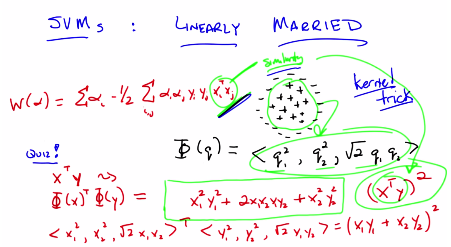
C: Okay? All right. Now, why did I do this? I did this because it’s going to turn out to provide a cute little trick. And in order to see that cute little trick we need to return to our quadratic programming problem. So let me remind you what that equation was. All right, Michael. So I’ve written up the equation for you, as I promised I would remind you, of the quadratic program that we’re trying to solve. I didn’t write down all of the constraints and everything. I’m hoping that you remember them. And I wrote it up there for a reason. And the reason I wrote it up, is because you’ll recall, just not too long ago, I asked you to talk about Xi and Xj , and what it looks like in this equation. And what I think we agreed to, or at least I know I agreed to, is that we can think about Xi transpose Xj as capturing some notion of similarity. So, it turns out then, if we sort of buy that idea of similarity, that really what matters most in solving this quadratic problem, and ultimately solving our optimization problem, is being able to constantly do these transpose operations. So, let’s ask the question that, if I have this new function, phi, what would happen if I took two data points, and I did the transpose or the dot product between them. What would I get? So, let me just write that out. Or, I don’t know, you can try telling me if you want to. So let’s make that, let’s make that let’s make that simple, Michael. And in fact, let’s make it so simple we can make it into a quiz.

Quiz: What is the Output?

scribble

• Move things into another dimension.

slides

transcript

C: Okay, Michael. Here’s a problem I want you to solve. Let’s imagine we have two points. I’m going to call them X and Y, just so I can confuse you with notation. And they are both two dimensional points. So they’re in a plane. And they have components X1 and X2 and components Y1 and Y2. Okay?

M: Sure.

C: And rather than computing the X transpose Y, their dot product, I want to compute the dot product of those two points, but passed through this function phi. You got it?

M: Yep

Answer

C: All right Michael, you got the answer?

M: I’m still carrying some squareds.

C: You want to talk it through?

M: Okay. Sure. So, x is really x1x2 and y is really y1y2 and phi x is now this crazy triple x so I, so I wrote x1 2x2 2 , square root of x1x2.

C: Yeah.

M: That’s the vector that we get for phi x. Then for phi y, I get y1, it seems like it would be helpful to see this.

C: You want me to write it down?

M: Sure.

C: Okay. So that turns out to be the same as what did you say? x1 2x2 2.

M: Root 2, x1, x2.

C: Root 2, x1, x2. Okay.

M: And then the y vector gets transformed to the same thing, except for with y’s, y1 squared comma, y2 squared comma, root 2, y1, y2.

C: Okay.

M: So, then, the, the dot product is just, the, the products of the corresponding components summed up. So x1 squared, y1 squared plus,

C: Okay

M: X2 squared, y2 squared,

C: Mm-hm

M: 2 x1, x2, y1, y2

C: That’s right. So here’s a question for you, Michael. Does that look familiar? Based on your years of thinking about algebra.

M: Oh, thanks for writing it that way! I see. We can, is this right? So it’s, it’s like, we can factor this.

C: Mm-hm.

M: It’s like x1 plus x2 times y1 plus y2.

C: Yeah, that’s right. Wait, is that right?

M: No it’s not right. X1 Y1

C: Mm-hm.

M: Plus X2 Y2. Whole thing’s squared.

C: Right. So, let’s write that down. So if you factor it out, you’re right, this is exactly equal to, X1

Y1 plus X2 Y2. Squared. And what’s an even simpler way of writing that? M: I see. x1 y1 plus x2 y2 looks like a dot product itself. It looks like the dot product of x and y. Oh, it’s x transpose y on the inside, and then we square it on the outside.

C: That’s exactly right. So now do you see why there was method to my madness when I created the phi function?

M: Not yet. So you’re saying, if we’re just dealing with dot products, now I’m still a little confused. So, so it is the case, that you define these in an interesting way, so that the dot product became the square of the old dot product.

C: Right, so now let me make two observations. Okay. Here’s observation one. What’s x transpose y? I mean geometrically, what does that represent?

M: The length of the projection of y onto x.

C: No I mean geometrically, like go all the way back to geometry, third grade.

M: We didn’t do transposes in third grade. [LAUGH]

C: I know we didn’t do transposes, but you did equations like this, or at least later you learned they were equations like this. Here, pretend you’re in third grade, and I said talk to me about geometry. What kind of words would you use?

M: Oh, what’s in geometry? Triangles. Circles.

C: Yeah. Circles! Did you say circles?

M: Sure, but only because I thought you might have wanted me to.

C: Did you say circles?

M: That’s a really ugly looking circle, sure.

C: Sure. This is basically a particular form of the equation for a circle Which means that we’ve gone from thinking about the linear relationship between Xi and Xj or your data points and we’ve now turned it into something that looks a lot more like a circle.

M: Interesting.

C: So if and this is my second point, Michael. If you believe me in the beginning where we notice that Xi transpose Xj is really about similarity. It’s really about why it is you would say two points are close to one another or far apart from one another. By coming into this transformation over here, where we basically represented the equation for a circle, we have now replaced our notion of similarity from being this very simple projection to being the notion of similarity is whether you fall in or out of a circle.

M: So more sort of about the distance as opposed to what direction you’re pointing.

C: Right, and both of them are fine because both of them represent some notion of similarity, some notion of distance in some space. In the original case, we’re talking about two points that are lined up together. And over here together with this particular equation we represented whether they’re inside the radius of a circle or outside the radius of a circle. Now this particular example assumes that the circle is centered at the origin and so on and so forth, but the idea I want you to see is that we could transform all of our data so that we separated points from within one circle to points that are outside of the circle. And then, if we do that, projecting from two dimensions here into three dimensions, we’ve basically taken all of the pluses and moved them up and all of the minuses and moved them back, and now we can separate them with the hyperplane.

M: Without knowing which ones are the pluses and which ones are the minuses, of course.

C: Of course.

M: Because, I see, because they are the ones that were closer to the origin.

C: Right.

M: So they get raised up less. Wow. Okay. So using that third dimension.

C: Right. Now, this is a cute trick, right? I can basically take my data, and I transform it into a higher dimensional space, where suddenly I’m now able to separate it linearly. That’s very cute, but I chose this particular form for a reason. Can you guess why?

M: Because it fits the circle pattern that you wanted.

C: But there are lots of different ways we could have fit the circle pattern. I chose this particular form because not only does it fit the circle pattern, but it doesn’t require that I do this particular transformation. Rather than taking all of my data points and projecting them up into three dimensions directly, I can instead still simply compute the dot product and now I take that answer and I square it.

M: So you’re saying in this formulation of the quadratic program that you have there in terms of capital W if you write code to do that, each time in the code you want to compute Xi transpose times Xj, if you just squared it right before you actually used it, it would be as if you projected it into this third dimension and found a plane?

C: Yes, that’s exactly right.

M: That’s crazy.

C: It’s so crazy it has a name. And that is the kernel trick. So, again if we really push on this notion of similarity. What we’re really saying is we care about maximizing some function that depends highly upon how different data points are alike, or how they are different. And simply by writing it this particular way, all we’re saying is, you know what, we think the inner product is how we should define similarity. But instead, we could use a different function altogether, phi or more nicely represented as x transpose y squared, and say, that’s our notion of similarity. And we can substitute it accordingly.

M: So we never really used phi.

C: We never used phi. We’re able to avoid all of that by coming up with a clever representation of similarity. That just so happened to represent something, or could represent something in a higher dimensional space.

M: So is it important that such a phi exists? Or is it just the case that we can, you know, we could, we could throw in a cubed, we could throw in a fourth, we could do a square root and a log, like can we do anything we want there in that Xi transpose Xj? Or are we constrained to only use things that somewhere out there, there is a way of representing it as a regular dot product?

C: Well, that is an interesting question. The answer is you can’t just use anything, but in practice it turns out you can use almost anything. And the other answer to your question is, it turns out for any function that you use, there is some transformation into some dimensional space, higher dimensional space, that is equivalent.

M: Whoa.

C: Now, it may turn out that you need an infinite number of dimensions to represent it. But there is some way of transform, transforming your points into higher dimensional space that happens to represent this kernel, or whatever kernel you choose to use.

M: So, which part is the kernel?

C: So, the kernel is the function itself. So, in fact, let me, let me, let me clean up this screen a little bit. And, and see if we can make this a little bit more precise and easier to understand.

Kernel

scribble

• Specific Requirement for a kernel function to go through is called the Mercer Condition.

slides

transcript

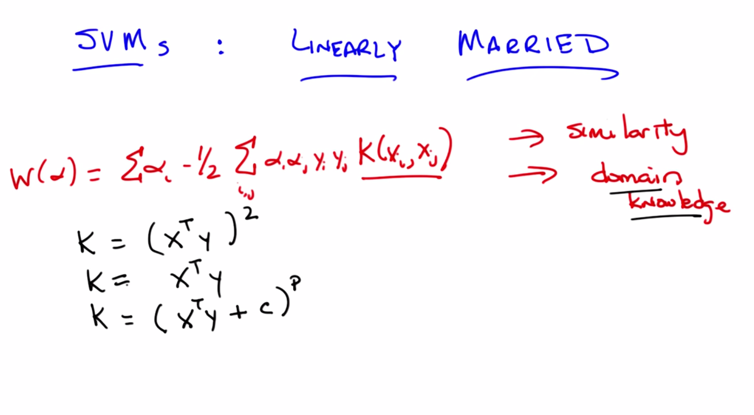
C: Okay, so I’ve the cleaned up the screen a little bit, Michael to, to make this a little bit clearer. Now, let’s look at this xi transpose xj. And I’m now going to replace it with something. So, I’ve just replaced it with a function, which I’m going to call a kernel. Which takes xi and xj as parameters, and will return some number. And again, as we talked about before, we think of the xi transpose xj, as some notion of similarity, and so this kernel function is our representation, still, of similarity. Another way of thinking about that, by the way, is that this is the mechanism by which we inject domain knowledge into the support vector machine learning algorithm.

M: Just like we were injecting domain knowledge when we were thinking about k-nearest neighbors.

C: Yes, everything has domain knowledge and everything ultimately comes back to k-nearest neighbors. I don’t know why and I don’t know how, but it always seems to.

M: So the k in k-nearest neighbors, and the k in kernel really stand for knowledge.

C: Oh, wow, that’s pretty good. We should write a paper with that title.

M: [LAUGH] So the room neatness here, the neatness here two fold. One is, you can create these kernels and these kernels have arbitrary relationships to one another. so, what you’re really doing is, projecting into some higher dimensional space, where, in that higher dimensional space, your points are in fact, linearly separable. But, the second bit is, because you’re using this kernel function to represent your domain knowledge, you don’t actually have to do the computation of transforming the points into this higher dimensional space. I mean, in fact if you think about it, with the last kernel that we used, computationally, there was actually no more work to be done. Before we were doing x transpose y, and now we’re still doing x transpose y, except we’re then squaring it. So that’s just a constant bit more work. Right?

C: So is, and that is a kernel and another kernel is X transpose Y?

M: Yes, that’s something I would call a kernel.

C: And the other kernel we talked about was just X transpose Y by itself. That’s, that’s a kernel too, isn’t it?

M: Oh no, no. That’s right. That’s right. That’s absolutely right. So, that’s a different kernel, you’re absolutely right. Just X transpose Y. Is another kernel. Actually we can write a general form of both of these. And as a very typical kernel, it’s the polynomial kernel where you have x transpose y plus some constant, let’s call it c, raised to some power p. And as you can see, both of those earlier kernels are, in fact, just a special case of this.

C: Hm, and I would, yeah, okay, good.

M: And that should look familiar.

C: It reminds me of the regression lecture.

M: Exactly, where we were doing polynomial regression. So now, rather than doing polynomial regression the way we were thinking about it before, we use a polynomial kernel and that will allow us to represent polynomial functions. And there’re lots of other kernels you can come up with, Michael. So. Here’s just a couple. I will just sort of leave em. Leave em up to you, to think about. And there’s, there’s tons of them. So, here’s one that I, I happen to like. So, that’s a a sort of, radial basis kernel. Does that look familiar to you?

M: Well, to me, make sure I understand that it’s doing the right thing. So if x and y are really close to each other, then it’s like, e to the minus zero over something which is like e to the zero, which is like one. So there’s similarities like one if they’re on top of each other. If they’re very far apart, then it’s like their distance is something very big divided by something e to the minus something very big is very close to zero. So it does have that kind of property kind of like the sigmoid where it, it transitions between zero and one but it’s not exactly the same shape as that.

C: Right in fact it’s symmetric, that the square of the of the distance between you in making an actual distance, makes it always a positive value there. Or at least a non-negative value there. And so it becomes symmetric, so it looks a lot more like a, like a gauchon with some kind of width which is represented by sigma. And there are tons and tons of these. Actually if you wanted to get something that looked like a sigmoid, here’s one. Where alpha’s different from the other alphas, but I couldn’t think of a different Greek letter. And this function gives you something that looks a lot more like a sigmoid. And there’re tons and tons of these you can come up with. And there’s lots of, been a lot of research over the years on what makes a good kernel function. The most important thing here, I think, is that it really captures your, your domain knowledge. It really captures your notion of similarity. You might notice, Michael, that since it’s just an arbitrary function that returns a number, it means that X and Y or the, the different data points you have, don’t have to actually be points in a numerical space. They could be discrete variables. They could describe whether you’re male or female. As long as you have some notion of similarity to play around with, that you can define, that returns a number, then it doesn’t matter. It will always work.

M: So can you do things like, I don’t know, strings or graphs or images?

C: Absolutely. You could think about two strings. How are two strings similar? Maybe they’re, they’re similar if their edit distance is small. The number of transformations that you have to give in order to transform one string to another. If there are few of those, then they’re very similar. If there are a lot of those then they’re very dissimilar.

M: All right. But then I, then I think I understand.

C: Okay. Good. So you might be curious, Michael, whether there are any bad kernel functions. There is actually an answer to that. While it’s not clear whether there are any bad kernel functions, it is the case that in order for all the math to go through, there is a specific technical requirement of a kernel function. It has a name. And it’s the Mercer Condition. Have you ever heard of the Mercer Condition?

M: I’ve heard the word. I actually used to live near Mercer County in New Jersey.

C: You did?

M: Yeah.

C: Oh. So then I guess it’s the condition of living near where Michael used to live. Now, so the Mercer condition is a very technical thing we’ll talk about this again, a little bit in the homework assignment. But for your intuition in the meantime, it basically means it acts like a distance, or it acts like a similarity. It’s not an arbitrary thing that doesn’t relate the various points together. Being positive is something definite in in this context means it’s a well behaved distance function.

M: Gotcha.

Summary of SVM

scribble

slides

Back to Boosting

scribble

• In K Nearest Neighbours, variance is a stand in for confidence. Low variance means everyone agrees, high variance means there is some disagreement.

slides

transcript

C: Alright, so back to boosting, Michael. So as you recall the little teaser I left you with last time, is that it appears that boosting does not always over-fit. And a little graph. That’s true, but it doesn’t seem to over-fit in the ways that we would normally expect it to over-fit. And in particular we’d see a, you know, an error line on training And what we expect to see is a testing line that would, you know, hue pretty closely and then start to get bad. But what actually happens is that instead, this little bit at the end where you get over fitting seems to instead. Just keep doing well. In fact, getting better and better and better. And I promised you an explanation for why that was. So, given what we talked about with support vector machines, and what we spent most of our time thinking about, what do you think the answer is?

M: Well I, I don’t think I would have asked again if I, had a thought about it. But you mean you want me to connect it to support vector machines, somehow. Well the, the thing that was fighting over fitting in support vector machines, was trying to focus on maximum margin classifiers.

C: Here, let me, let me try to explain to you why it is that you don’t have this problem with overfitting at least not in the, in the typical way as you keep applying it over and over again like you do with something like neural networks. And it really boils down to noticing that we’ve been ignoring some information. So, what we normally keep track of is error. So error on say a training set is just, you know, the probability that you’re going to come up with an incorrect answer or come up with an answer that disagrees with your training set. and that’s a very natural thing to think about and it makes a lot of sense. But there’s also something else that is actually captured inside of boosting and captured by a lot of learning algorithms we haven’t been taking advantage of, and that’s the notion of confidence. So confidence is not just whether you got it right or wrong. It’s how strongly you believe in a particular answer that you given. Make sense?

M: Yes, a lot of the algorithms we talked indirectly have something like that. So, like in a nearest neighbor method, if you are doing five nearest neighbor and all five of the neighbor agree, that seems different than the case with vote one way and two vote the other.

C: Right. And in fact, that’s a really good example. If you think of that in terms of regression Then you could say something like the variance, between them is sort of a stand in for confidence. Low variance means everyone agrees, high variance means, there’s some major disagreement. Okay. So what does that mean in the boosting case? Well as you recall, the final output of the boosted classifier is given by a very simple formula. And here’s the equation here that h of x is equal to the sine of the sum over all of the weak hypothesis that you’ve gotten of alpha times h. So the weighted average of all of the hypothesis, right? And you just simply, if it’s positive you produce a plus one. And if it’s it negative you produce a minus and if it’s exactly zero you don’t know what to do so you just. Produces zero. Just throw up your hands. So I’m going to make a tiny change to this formula, Michael. Just, just for the purpose of sort of, explanation, that doesn’t change the fundamental answer. And I’m just going to take exactly this equation as it is. And I’m going to divide it, by the weights that we use. Now what does that end up doing?

M: Okay, so the weights. I’m getting a. There’s Alphas in the SVM’s too, so I’m getting a little confused. So that I’m. I think these Alphas all have to be non-negative.

C: Right.

M: But they kind of like this support vector values, in that there could be zero, if, if that hypothesis isn’t come into play?

C: Well, but they want in that case, the, the alpha is always set to be the natural log of something.

M: Oh, oh, oh, and also these alphas are applied to hypothesis whereas the alphas in the, in the SVM settings were being applied to data points.

C: That’s right. So, unfortunately in machine learning, people in, invent things separately and reuse notation. Alpha’s an easy Greek character to draw, so people use it all the time. But here, remember, alpha’s the measure of how good a particular weak hypothesis was, and since it has to do better than chance, it works out that it will always be greater than zero.

M: Gotcha, okay. So this, this normalization factor, this denominator doesn’t, it’s just a constant with respect to x, the input. So it won’t actually change the answer. So it really is the same answer as we had before, just a different way of writing it.

C: Right. And what it ends up doing like often is the case in these situations, is it normalizes the output. So it turns out that this value. Inside here is always going to be between minus one and plus one. Okay? But otherwise it doesn’t change anything about what we’ve been doing for boosting. So you might ask why did I go through the trouble of normalizing it between minus one and plus one?

M: Why indeed?

C: Well it’s makes it easier for me to draw what I want to draw next. So, we know that the output of this little bit inside the sign function is always going to be between minus one and plus one. Let’s imagine that I take some particular data point x and I pass it through this function, I’m going to get some value between minus one and plus one. And let’s just say for the sake of the argument, it ends up here. Okay?

M: Is that an x or a plus?

C: That’s a plus.

M: Okay. So it’s a positive example and it’s near plus one.

C: Right.

M: So this would be something that the algorithm is getting correct.

C: Yes, and it’s not just getting it correct, but it is very confident. In its correctness. because it gave it a very high value. By contrast there could have been another positive that ends up around here.

M: Hmm.

C: So it gets it correct but it doesn’t have a lot of confidence so to speak in its correct answer because it’s very near to zero. So that’s the difference between error and confidence. Because for example I could also have a plus value way over here. So I am very, very confident in my very, very incorrect answer.

M: Mm.

C: So this is my daughter, for example. [LAUGH] She’s very confident whether she’s right or wrong. [LAUGH] Okay. And so now imagine there’s lots of little points like this. And if you’re doing well, you would expect that, you know, very, very often you’re going to be correct. And so you end up shoving all the positives over here to the right, and all the negatives over here to the left. And it would be really nice if you were sort of confident in all of them. Okay, so does this make sense, Michael as a picture,

M: Oh yeah. What, what might be going on? Absolutely.

C: Okay, good. So now I want you to imagine that we’ve been going through these, these training examples, and we’ve gotten very, very good training error. In fact, let’s imagine that we have negative training error. I’m [LAUGH]

M: Wow.

C: In fact, let’s imagine that we have no training error at all. So we, we label everything correctly. So then the picture would look just a little bit different We’re going to have all the pluses on one side, and all the minuses on the other. But we keep on training, we keep adding more and more weak learners into the mix. So here’s what ends up happening in practice, right? What ends up happening in practice is, you have to do some kind of distribution on the hard examples. And the hard examples are going to be the one that are very near the boundary. So as you add more and more of these weak learners what seems to happen in practice is that these pluses that are near the boundary and these minuses that are near the boundary just start moving farther and farther away from the boundary. So, this minus starts drifting and drifting and drifting until it’s all the way over here, this minus starts drifting and drifting and drifting untili it’s all the way over here. And the same happens for the pluses. And as you keep going and you keep going, what ends up happening is that your error stays the same. It doesn’t change at all, however your confidence keeps going up and up and up and up and up. Which has the effect, if you’ll look at this little drawing over here of moving the pluses all around over here, so they’re all in a bunch, and the minuses are on the other side. So what does that look like to you, Michael?

M: This picture?

C: Yeah.

M: I mean that there’s a, there’s a big gap between the leftmost plus and the right most minus. Which, you know, in the context of this lecture reminds me of a margin.

C: That’s exactly right. Basically what ends up happening is that as you add more and more weak learners here the boosting out rhythm ends up becoming more and more confident in its answers which it’s getting correct. And therefore effectively ends up creating a bigger and bigger margin. And what do we know about large margins?

M: Large margins tend to minimize overfitting.

C: That’s exactly right. So it, counter intuitively, as we create more and more of these hypotheses, which you would think would make something more and more complicated, it turns out that you end up with something smoother, less likely to overfit and ultimately, less complicated. So the reason boosting tends to do well and tends to avoid overfitting even as you add more and more learners is that you’re increasing the margin. And there you go. And if you look in the reading that we gave the students there’s actually a detailed description about this in a proof.

M: Cool.

C: Okay. So, there you go, Michael. Do you think, then, that boosting never overfits?

M: Never seems like such a strong word. I mean, the story that you told says that it’s going to try to separate those things out, but I guess I guess it doesn’t have to be able to do that. I mean, it could be that for example all the weak learners are I dunno very unconfident very inconsistent.

C: Hm. Okay, well you know, maybe, maybe it’s worthwhile to take a little diversion here to take a five second quiz.

Quiz: Boosting Tends to Overfit

scribble

slides

transcript

C: Okay Michael. So here’s a quick quiz. So we just tried to argue that boosting has this annoying habit of not always overfitting, but of course something can always over fit. Because otherwise we just do boosting and we’re done, then neither of us would have jobs. And we don’t want that to happen. So here’s a little quiz to see if we can figure out the circumstances under which boosting might overfit, or tends to overfit. So here are five possibilities. Let me read them to you. Tell me if they actually make sense. So here’s possibility number one, boosting will tend to overfit if the weak learner that it’s boosting over, always chooses the weakest output that is, it, among all the hypothesis that it finds that do better than chance over the training with whatever given distribution. It always picks the one that is still nonetheless closest to chance, while still being better.

M: Well, why would it do that?

C: Just to be difficult. Alright, and so you want to know, whether that makes it over, would make it over fit?

M: Okay. Alright.

C: The second one is the weak learner actually ends up using…or the weak learner itself that boosting is using is in fact a neural network learner. And just for a little specificity, let’s say this is a neural network that has many many layers and many many nodes. So, you know, it’s a big powerful neural network, alright? the other option is… boosting has a lot of data. So you’re trying to learn, your training data is actually very, very, very large. You have lots and lots of examples. The fourth case, is that, the true underlying hypothesis,the true underlying concept, is in fact non linear. So you can’t just draw a line. And then the fifth case is that we let boosting train much too long. Whatever that means. Let’s just say we let it train a lot. Not just a thousand iterations but a hundred billion iterations.

M: Okay.

Answer

C: All right, Michael. What’s the answer?

M: All right. Well, let me start off with what I think the answer isn’t. So, the last one, boosting tends to overfit, if boosting trains too long. You just told me a story about that not being true. So I’m going to eliminate that one from consideration. Boosting training too long.

C: Oh, nice to know you were listening.

M: [LAUGH] Boosting training too long, seems like not a good reason for it to overfit.

C: You’re correct.

M: All right. Boosting tends to overfit if it’s a nonlinear problem. So, that doesn’t seem right. I mean I guess, no, this one just doesn’t seem right at all. Like I don’t see why, why the problem being linear or nonlinear, has anything to do with overfitting.

C: Okay.

M: A whole lot of data is the opposite of what tends to cause overfitting. If there’s lots of data then you’d think that it would actually do a pretty reasonable job of, you know, there’s a lot to fit. There’s a lot going on there. It’s unlikely to overfit.

C: Right, and in fact if a whole lot of data included all of the data, and you actually could get zero training error over it, then you know you have zero generalization error because it’ll work on the testing data as well, because it’s in there.

M: Right.

C: All right. Weak learner uses artificial neural network with many layers and nodes. So I’m guessing that you wanted me to think about that being something that, on its own, is prone to overfitting, because it’s got a lot of parameters.

M: Sure.

C: So, if, and now we’re doing boosting over that. So we fit a neural net, and then we fit another neural net, and we fit another neural net. And we’re combining all the outputs together in the correct, weighted way. It’s not obvious to me that that should be a good thing to do. I’m not sure it would overfit, but it seem like it sure could.

M: OK, so you’re, so for now let’s put a little question mark to it. You think that might be the right answer, but you want to think about it some more?

C: Yeah let me look at the first one. Weak learner chooses the weakest output. Well, I mean boosting is supposed to work as long as we have a weak learner. And it doesn’t matter if it chooses the weakest or the strongest. All that matters is it does significantly better than a half. So, like I feel like the only one, the only one of these choices that is likely to be true is the second one.

M: And that is, in fact, correct. So let me give you an example of when that would be correct. So let’s imagine I have a big powerful new network that could represent any arbitrary function. Okay, it’s got lots of layers and lots of nodes. So, boosting calls it, and it perfectly fits the training data, but of course overfits. So then it returns, and it’s got no error, which means all of the examples will have equal weight. And when you go through the loop again, you will just call the same learner, which will use the same neural network, and will return the same neural network.

So every time you call the learner, you’ll get zero training error, but you will just get the same neural network over and over and over again. And a weighted sum of the same function is just that function. So if it overfit, boosting will overfit.

C: Interesting. And not only will it overfit, but it’ll just, it’ll be stuck in a horrible loop of error.

M: Right. So that’s why this is the sort of situation where you can imagine boosting providing a lower fit. If the underlying learners all overfit and you can never get them to stop overfitting, then there’s really not much you can do.

C: Interesting.

M: Now, I do want to have a little semantic argument with you for a moment, Michael. You used the word strongest at some point, when you were talking about using the weakest output. And I just want to point out that, that doesn’t really mean anything.

C: What do you mean, it doesn’t mean anything?

M: Well, so what’s a strong, what would you call a strong learner?

C: One that is far away from it. If a weak learner just has to do a little bit better than a half, it seems like a strong learner would be something that would be very close to being accurate.

M: Right. Of course, on the other hand, if by that definition all strong learners are also weak learners.

C: Sure.

M: Because anything that does better than a half is still doing better than a half, which is all it requires to be a weak learner.

C: Yeah, but that’s kind of true of people too. Like a strong person is also a weak person.

M: No.

C: Well it depends how you define it. So, if you say a weak person is someone who can at least lift their own arms, then strong people are also weak people in that they can lift their arms.

M: Yes if you define it that way and if I define blue to be purple, then I can say blue is purple. But that’s not how people define weak people. They define weak people, by saying they can’t lift more than, not that they can lift at least as much.

C: I see. So it’s this piece of terminology that boosting uses that is in error, not me.

M: That’s one interpretation. It’s not the one that I would use, but it’s one interpretation. When you say something like a strong learner, I mean, it makes sense to use that kind of term, and sort of throw it around, and say, well, by a strong learner I mean someone who’s, or a learner that’s going to overfit, or is going to always do really well on the training data. But in kind of a technical definition it’s very difficult to sort of pin down. So don’t get too caught up what a strong learner means if you want to write a proof. Seems fair?

M: Good point yeah, also, also that this whole notion that strong is sometimes defined as not weak. And it is not the case that if you have something that’s not a weak learner that it’s, then it’s a strong learner. In fact, it’s no learner, no learner at all.

C: Exactly. So, a weak learner’s just defined in a way that basically says, it gives me at least some information. Good. Let me just throw one more thing in here and then we can stop talking about this. There’s another, a couple of other cases where boosting tends to overfit. The one that matters the most, or comes up the most, is in the case of pink noise.

M: Did you say, peak noise?

C: I said, pink noise. I even wrote it in red, which looks like pink. It’s a strong pink as opposed to a weak pink.

M: I’m sorry. There’s no way for that to be obvious from what we’ve talked about, but as a practical matter, pink noise tends to, cause boosting overfit.

C: Okay, but this is not a term I’m familiar with unless you’re critiquing the musical stylings of a particular performer.

M: [LAUGH] No. Although I did recently see, see them in concert. But that’s a whole other conversation. Okay, so pink noise just means uniform noise.

C: I thought white noise was uniform noise.

M: No, white noise is Gaussian noise. Okay, so pink noise is uniform noise and white noise is Gaussian noise. This is why, Michael, by the way, if you ever try to set up a studio or a cool stereo system in your house, you want a pink noise generator. So that it covers all the frequencies equally, not just the white noise. generated.

C: Hm.

M: But boosting tends to overfit in those sorts of circumstances. And you can read more about it in the notes if you want to. But the one that I want I really want people to get is, that if you have an underlying weak learner that overfits, then it is difficult for boosting to overcome that. Because fundamentally you’ve already done all of your overfitting and it’s, there’s really not much for those things to do.

C: Okay. Got it?

M: Got it.