Probability

Introduction

Decomposition

• Whenever we see a conditional probability, the first thing we look at is Bayes rule.

• We have to find out the probability of Y being True.
• At this point, we think of Venn Diagrams.

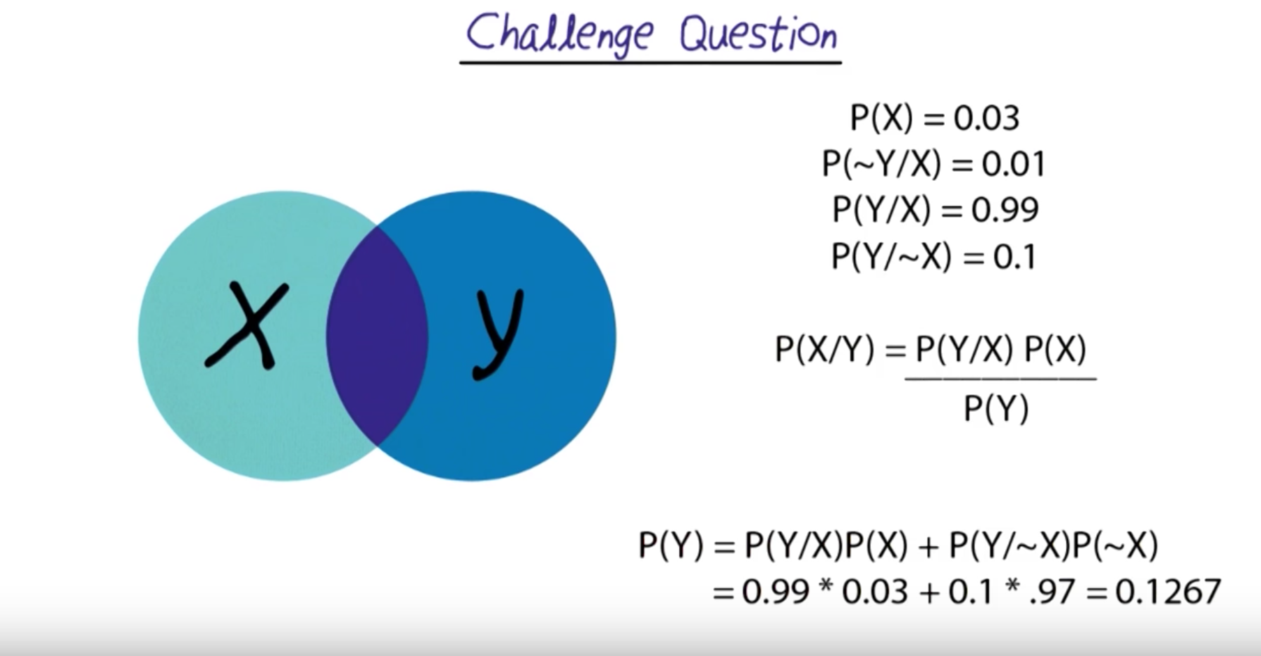
• Final calculation

Strategy

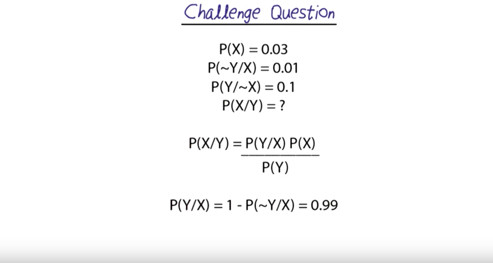
• Accurate Translation of the english into probability

P (X) = 3% = 0.03
P (-Y | X) = 1% = 0.01
P (Y | -X) = 10% = 0.1

P( X | Y) = ?

          = P (Y |X ) * P (X)
            -----------------
                 P (Y)

P (Y | X ) = 1 - P (-Y | X)
           = 1 - 0.01
           = 0.99


P ( Y ) = P ( Y |X) * P(X) + P(Y | -X) * P(-X)
         = 0.99 * 0.03 + 0.1 * (1-0.03)
         = 0.1267

P ( X | Y ) = 0.99 * 0.03 / 0.1267
            = 0.23441199684293604

Intro to Probability and Bayes Network

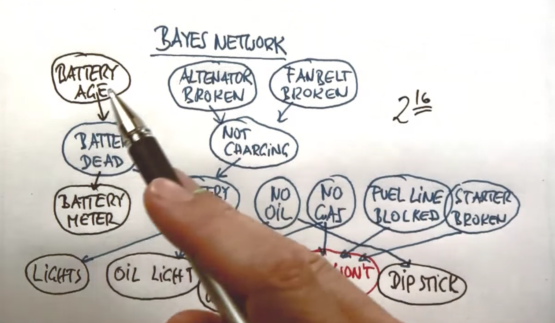
Bayes network is a compact representation of distribution of this very very large giant probability distribution of all these variables.

Using Bayes network, we have observe the probabilities of some variables and compute hypothesis of the probability of other variables.

Probability Summary

• Probability of Independent Events = Product of the Probability of Marginals
• Independent Events

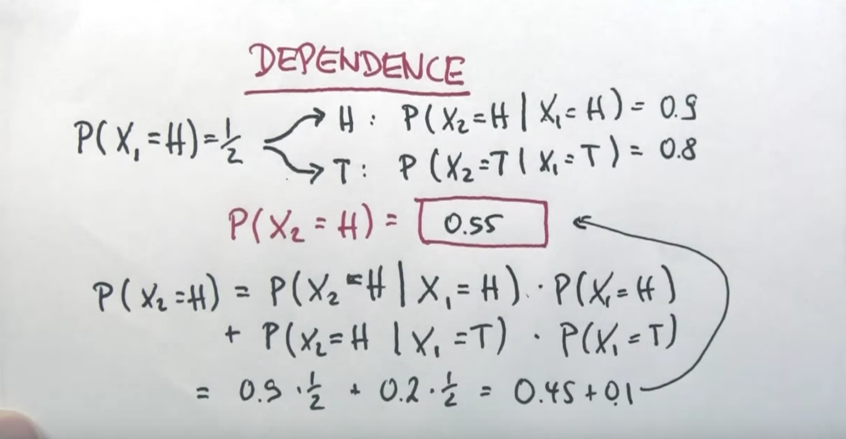
Dependence

• I will use the term “given that” for describing the condition after the “|”

• Theorem of Total Probability

What We Learned

• Total Probability
• Probability of any random variable Y, can be written as, Probability Y, “given that” some other random variable \(X_i\) , times \(P(X_i)\) , summed over all possible outcomes of i for the random variable X.
• Negation of Probability
• P(-X | Y) = 1 - P( X | Y)

• Can never negate the conditional variables and assume that it will add up to 1.

Weather Quiz

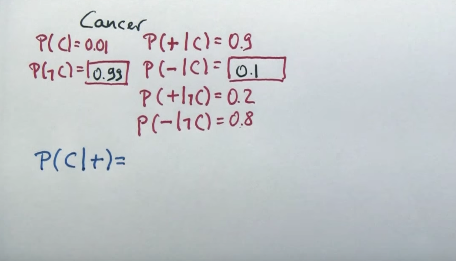
Cancer Example

• Before we calculate this, we are calculating the joint probabilities.
• Why are we calculating the joint probabilities?

Now, the joint probabilities are not independent events. They are joint probabilities of dependent events.

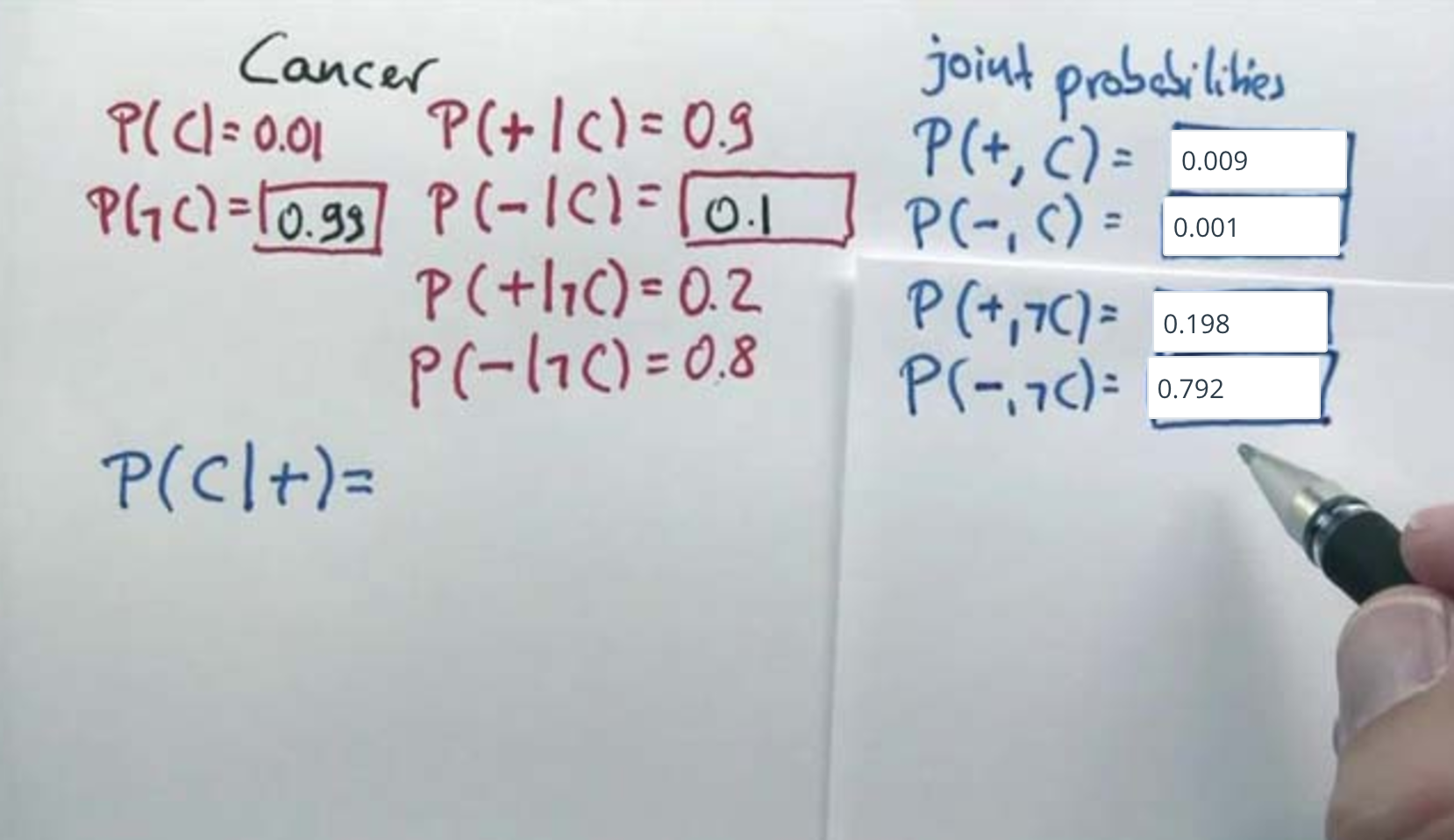
• The product of prior and the conditional

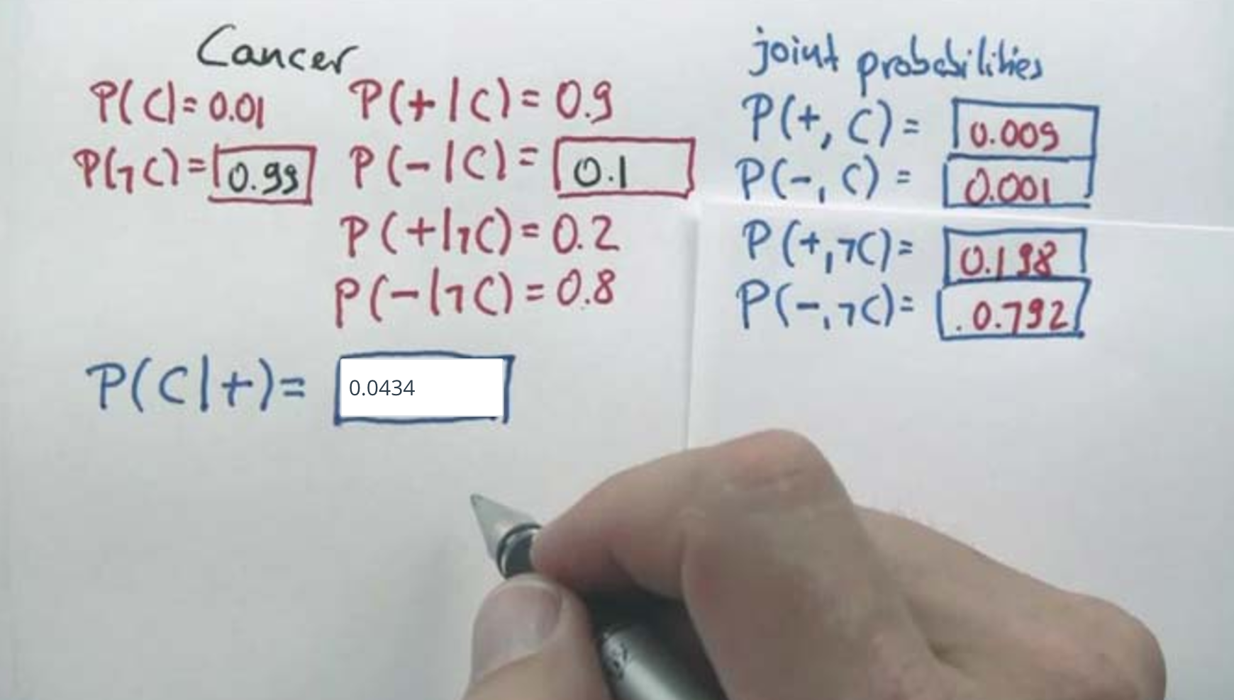
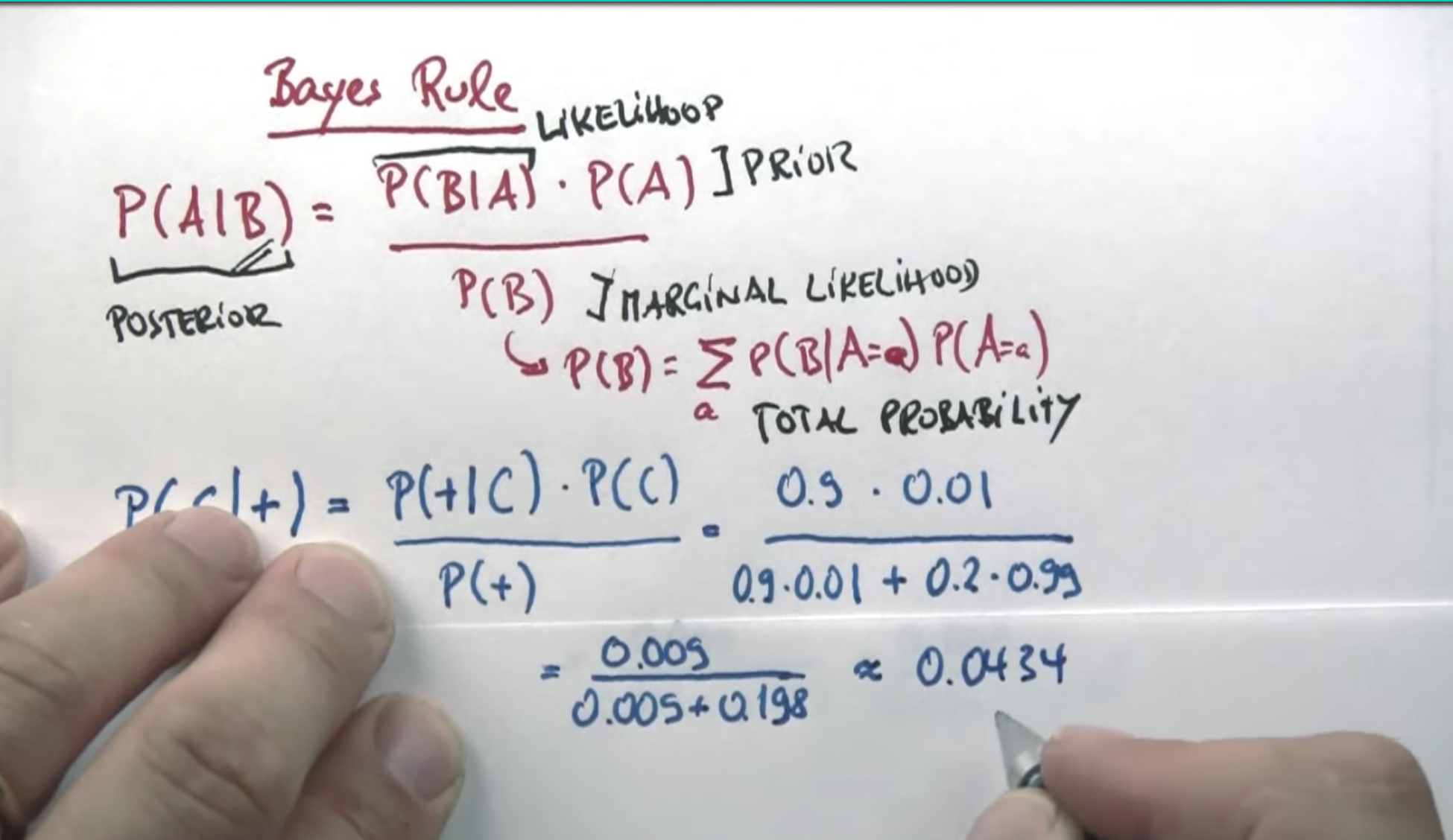
• We expand via Bayes Rule

P (C | +) =  P ( + | C ) . P ( C)  / P ( + )

          =  (0. 9 *  0.01) /  (0.009 + 0.198)
          =  (0.9 * 0.01)  / 0.20700000000000002
          = 0.043478260869565216o

• Not using the term “Total Probability” for the P(+), but essentially doing that.
• The prior for cancer is so small that it is unlikely to have cancer.
• The additional information of positive test, only raised the posterior probability to 0.043

Bayes Rule

• The most important maths for this class in statistics called Bayes Rule.
• B is the evidence.
• A is the variable we care about.
• For the variable we care about, we have a Prior
• For the expression with evidence, we say it as a marginal likelihood and likelihood for conditioned one.

• The evidence to cause, is turned into causal reasoning.
• Hypothetically given the cause, what is the probability of the evidence that just occurred. And to correct for this reasoning, we multiply it by the prior probability of the cause, and divide the whole by the normalized evidence.
• The Probability of Evidence is expanded often by the theorem of total probability.

Sum(forall a) P ( B | A = a)

Reference

• http://sites.nicholas.duke.edu/statsreview/probability/jmc/